| EE and EB spectra; effective rotation angle |
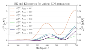 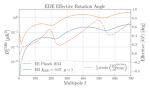 |
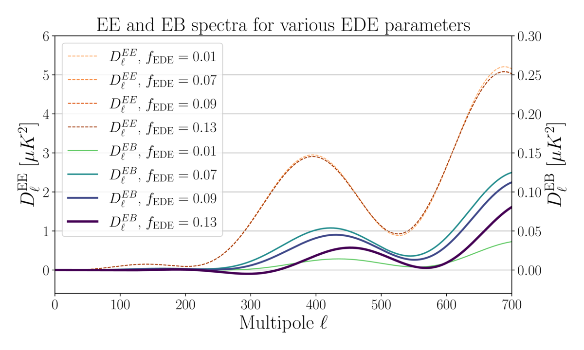
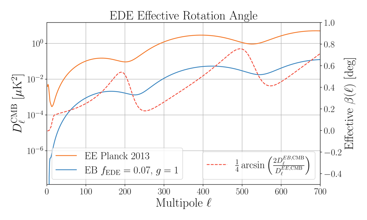
Figure 1: Multipole dependence in early dark energy. (Left) \(EB\) and \(EE\) spectra generated by early dark energy models with different values of \(f_\mathrm{EDE}\). As \(f_\mathrm{EDE}\) increases, the \(EB\) spectrum (blue) becomes more pronounced and deviates further from a constant rotation model, while the \(EE\) spectrum (orange) stays roughly the same. \(f_\mathrm{EDE}\) is the primary driver of these shifts, but other parameters (both EDE and standard cosmological parameters) also vary according to best fit values in Table I. Note the \(EE\) spectra and \(EB\) spectra are on different scales for visual comparison. (Right) Effective rotation angle (red) approximated by \(\beta(\ell) = \frac{1}{4} \arcsin \left( 2 D_\ell^{EB} / D_\ell^{EE} \right)\), where \(EB\) (blue) is derived from an EDE model with \(f_\mathrm{EDE} = 0.07\), and \(EE\) (orange) is the best fit curve from Planck 2013. Constant angle models are insufficient for fitting to \(\beta(\ell)\).
|
PDFa PDFb / PNGa PNGb |
| CMB spectra for isotropic vs. multipole-dependent rotation |
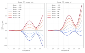 |
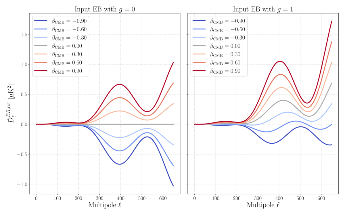
Figure 2: Comparison of simulated CMB spectra under isotropic vs. multipole-dependent rotation. (Left) Standard ΛCDM spectra rotation by different constant angles, \(\beta_\mathrm{CMB}\) (isotropic birefringence only, \(g = 0\)). (Right) Spectra including an early dark energy contribution (\(g = 1\)) rotated by different \(\beta_\mathrm{CMB}\). The EDE signal introduces distinct features in the \(EB\) spectrum that differ significantly from the isotropic case.
|
PDF / PNG |
| Histograms of jackknife statistics |
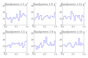 |
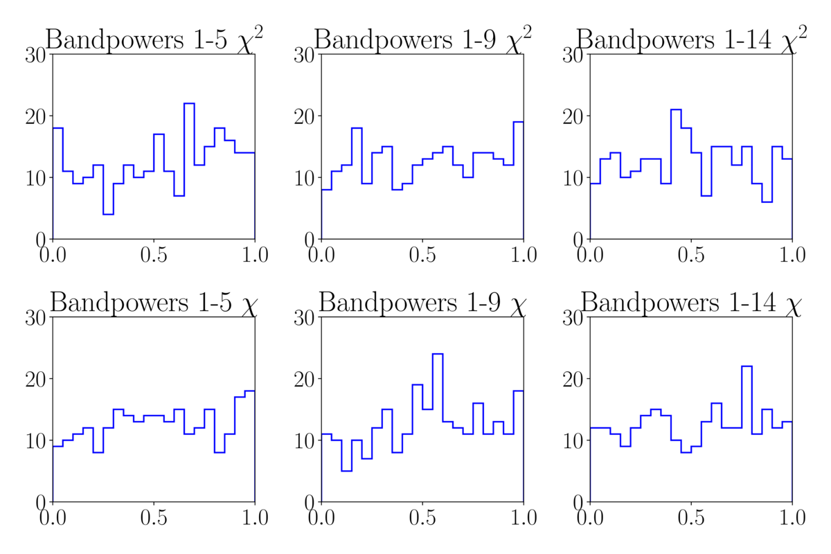
Figure 3: Distributions of the jackknife \(\chi^2\) and \(\chi\) PTE values for the Keck Array 2016, 2017, and 2018 220 GHz data. This figure is analogous to Fig. 12 of BK-XIII, but with an additional rightmost column showing the extended multipole range (band powers 1–14), explicitly checking that the higher multipole band powers also satisfy the jackknife consistency criteria.
|
PDF / PNG |
| Step function constraints |
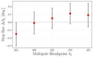 |
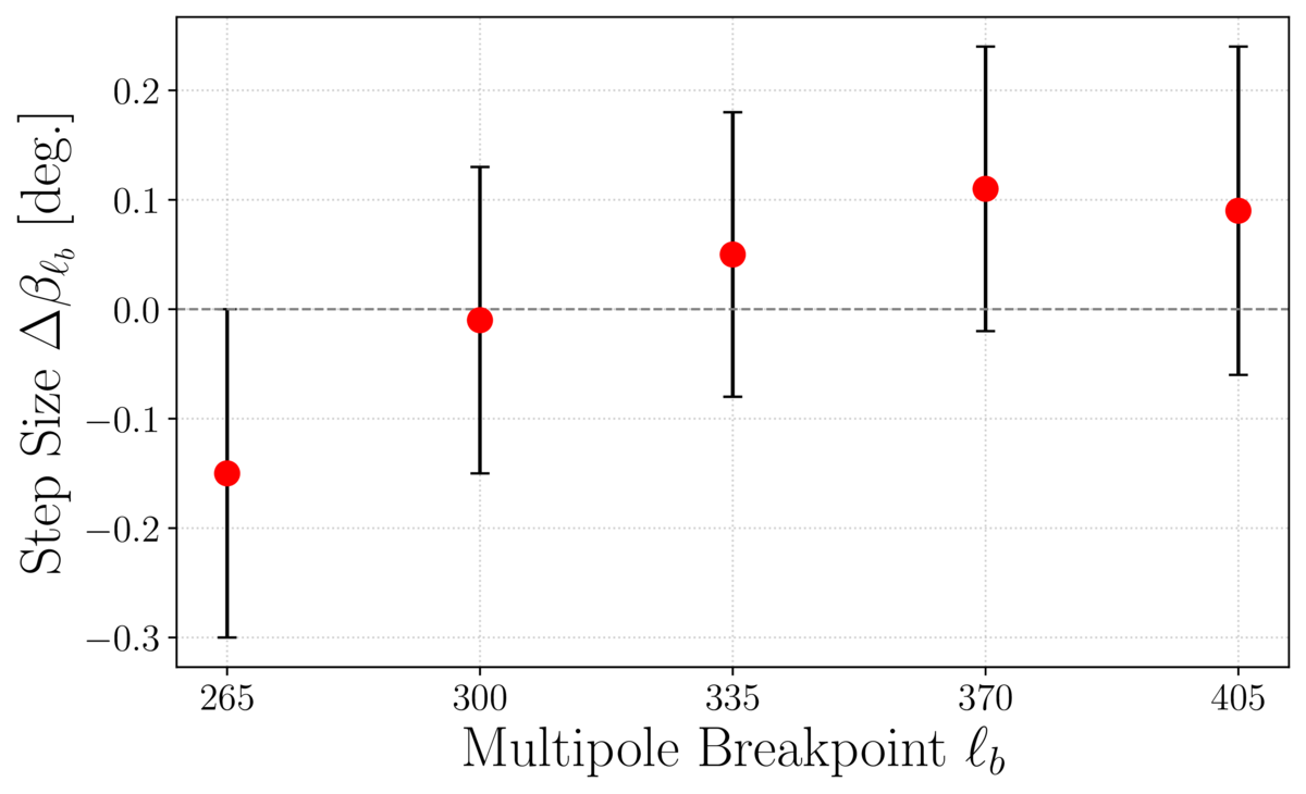
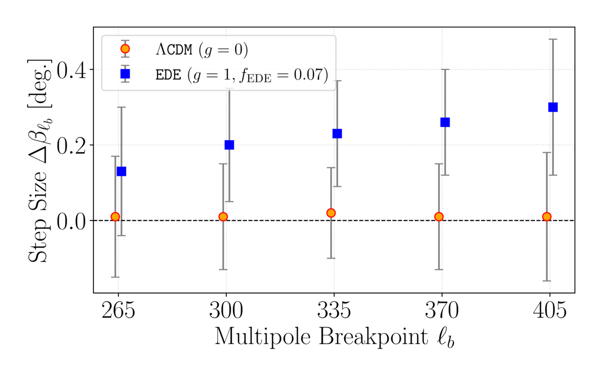
Figure 4: Best-fit \(\beta(\ell)\) step function for five values of the \(\ell_b\) breakpoints with \(1\sigma\) uncertainty. All values are consistent with \(\Delta\beta_{\ell_b} = 0\).
|
PDF / PNG |
| Early Dark Energy constraints |
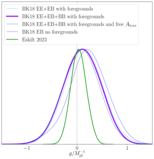 |
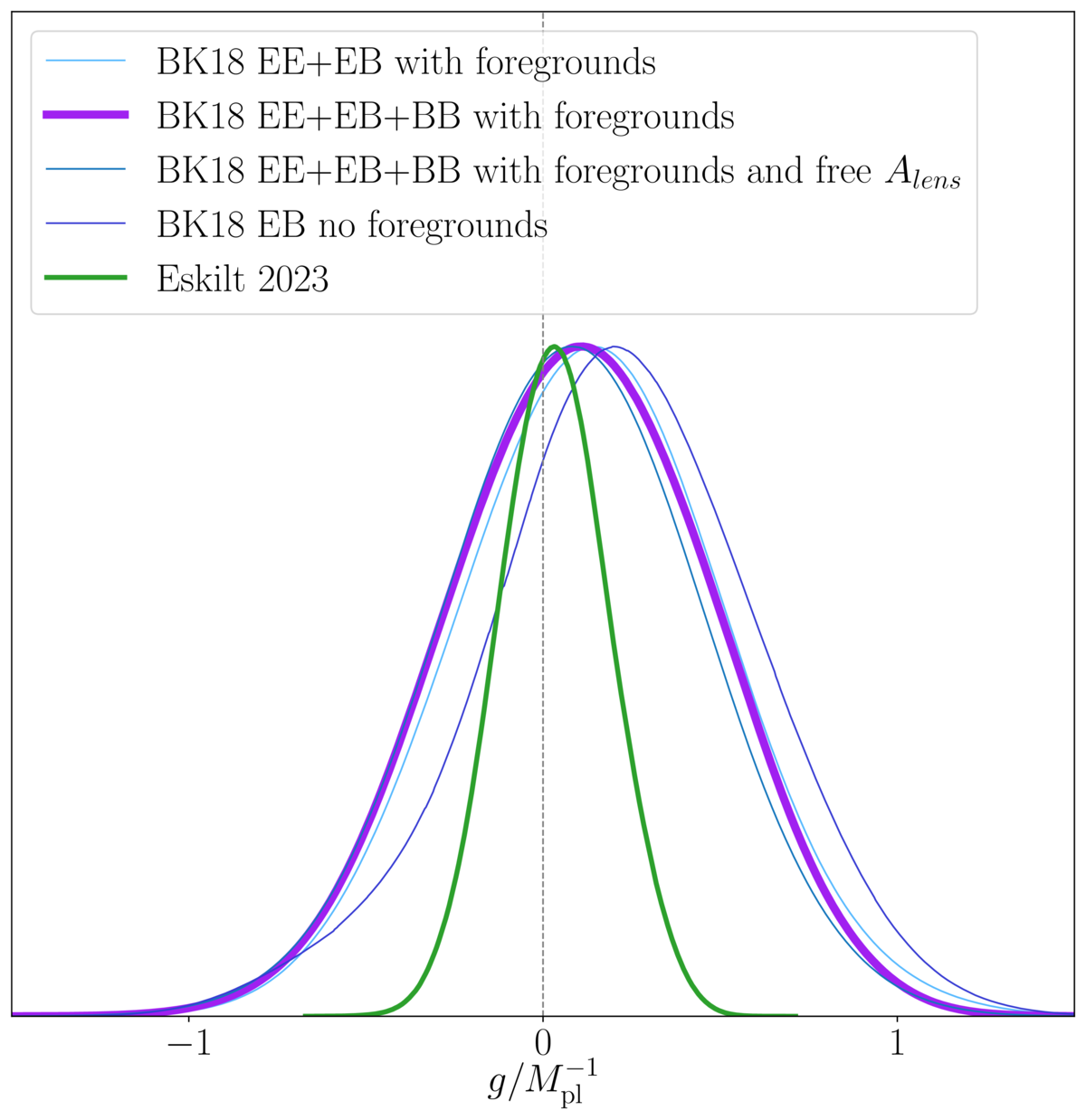
Figure 5: Posterior distribution on the axion-photon coupling \(g\) from BK18 (this work), overlaid with the constraint from Planck \(EB\) analysis by Eskilt et al. with the EDE parameters from their baseline result.
|
PDF / PNG |
| Visualizing \(\ell\)-dependent rotation |
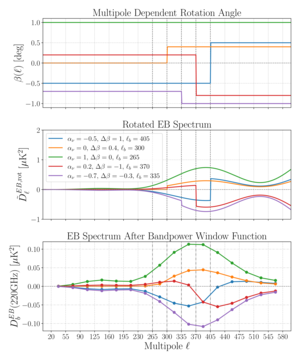 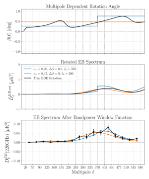 |
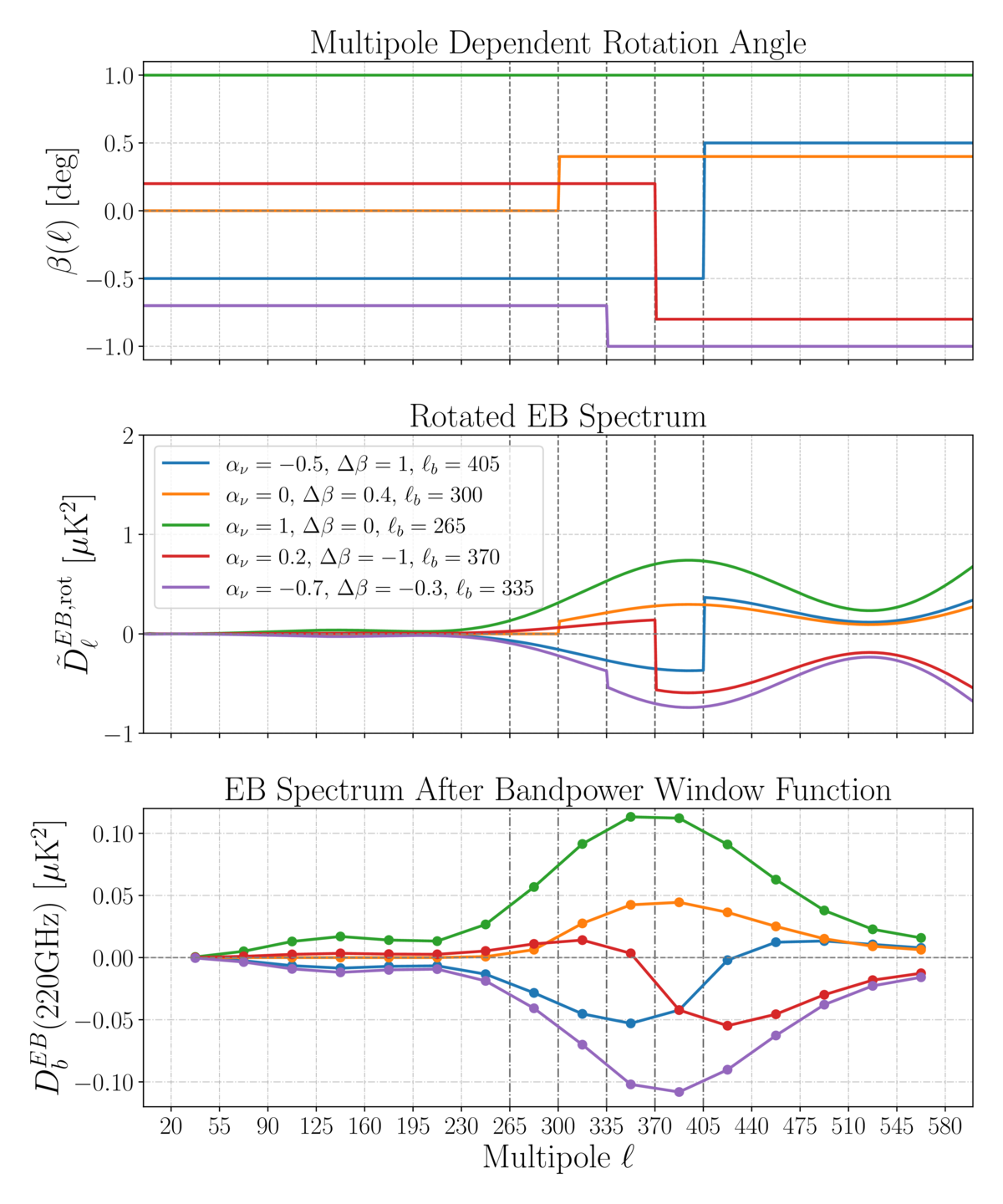
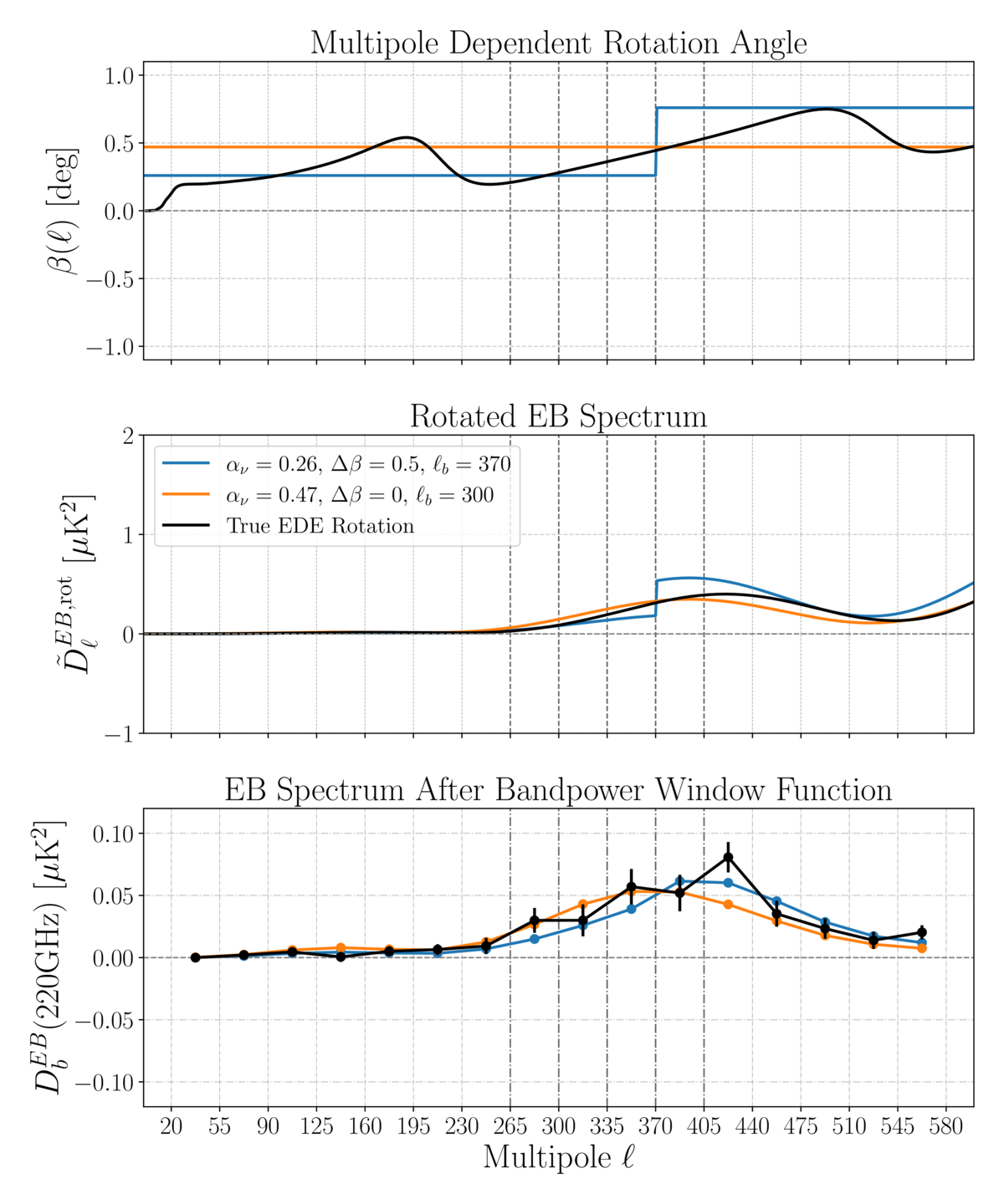
Figure S1: Visualizing step function modeling of \(\ell\)-dependent rotation. (a) Examples of \(\beta(\ell)\) modeled as step functions at various breakpoints \(\ell_b\). Each curve represents a different step size \(\Delta\beta_{\ell_b}\), demonstrating the effect of multipole-dependent changes in the polarization rotation angle. (b) Comparison between a step function \(\beta(\ell)\) model (blue) and a constant-angle model (orange), fit to simulated EDE \(EB\) data, sim 79 (black). To produce a marginally better fit (\(\chi^2\) = 17.1 vs 18.3), the \(\ell\)-dependent estimator accommodates the features in the data by recovering a significant step size over the constant rotation model. In both cases, \(g\) is set to zero so the \(EB\) spectrum is solely produced by this effective rotation.
|
PDFa PDFb / PNGa PNGb |
| Effect of band power window functions on power spectra |
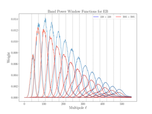 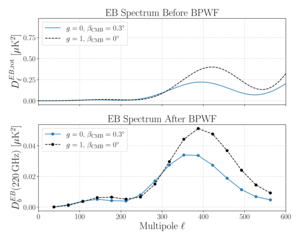 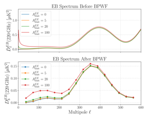 |
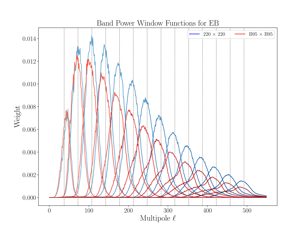
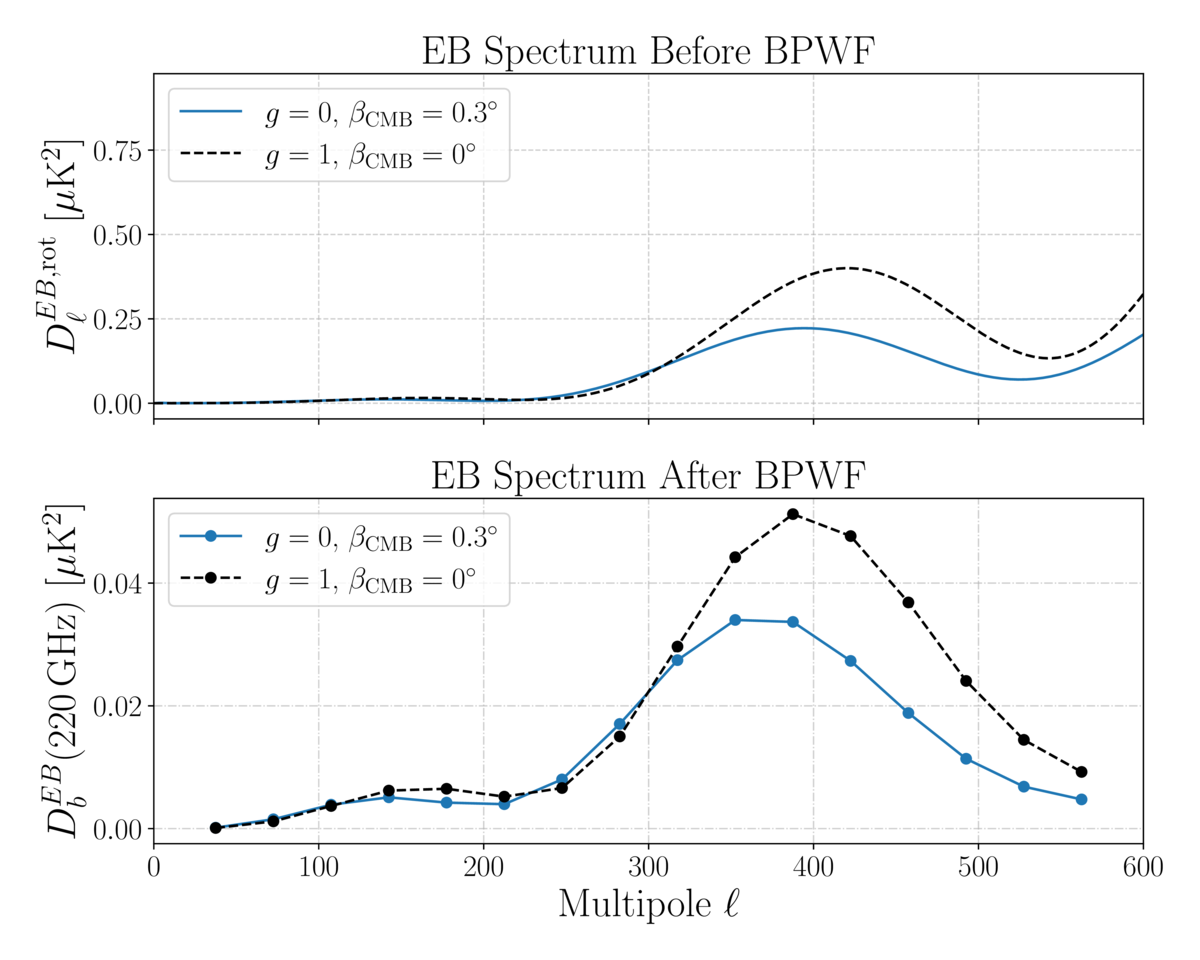
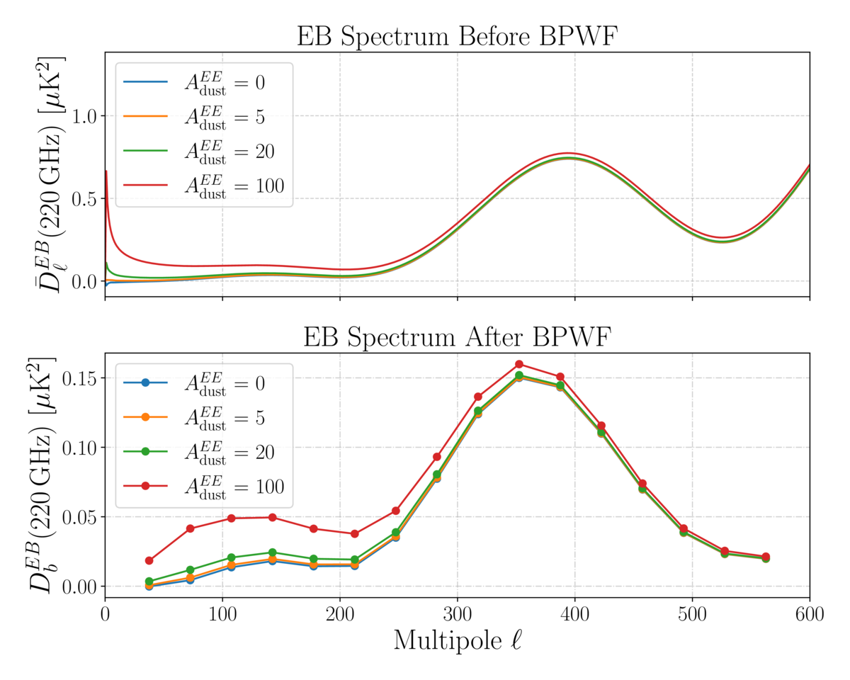
Figure S2: Visualizations of the Band Power Window Function and its effect on polarization spectra. (a) Band power window functions (BPWFs) for selected cross spectra, showing contribution to each band power across \(\ell\). Dashed lines correspond to nominal band power centers. (c) Effect of BPWF on \(EB\) spectra for varying \(g\) and \(\beta_\mathrm{CMB}\). No dust or per-band rotation applied. (d) Effect of BPWF on \(EB\) spectra with varying dust foreground parameters. Unspecified parameters are set to fiducial values (Table S2). Due to suppression factors from instrumental and analysis filtering, the binned spectra in the lower panels appear at a reduced amplitude relative to the theory spectra.
|
PDFa PDFc PDFd / PNGa PNGc PNGd |
| Validation of the model-independent step function estimator |
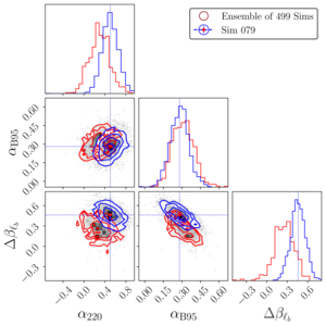 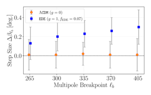 |
Figure S3: (a) Posterior distribution (where shaded regions represent 2D MCMC sample densities, and the contours represent the 68%, 95%, and 99% credible intervals) of the step amplitude \(\Delta\beta_{\ell_b}\) for a single EDE realization overlaid on the ensemble distribution of posterior means from 499 simulations (red). The blue dashed lines indicate the specific posterior mean for the representative realization (Sim 79), marking its position on the ensemble distribution with a red dot. (b) Recovered step amplitudes \(\Delta\beta_{\ell_b}\) across all tested multipole breakpoints. Points represent the average of the 499 posterior means, while error bars represent the 68% credible interval. The baseline set (blue) consistently recovers zero, while the EDE set (red) exhibits a nonzero, \(\ell\)-dependent signal characteristic of the injected birefringence.
|
PDFa PDFb / PNGa PNGb |
| Validation of parameter constraints for the EDE estimator |
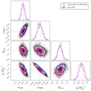 |
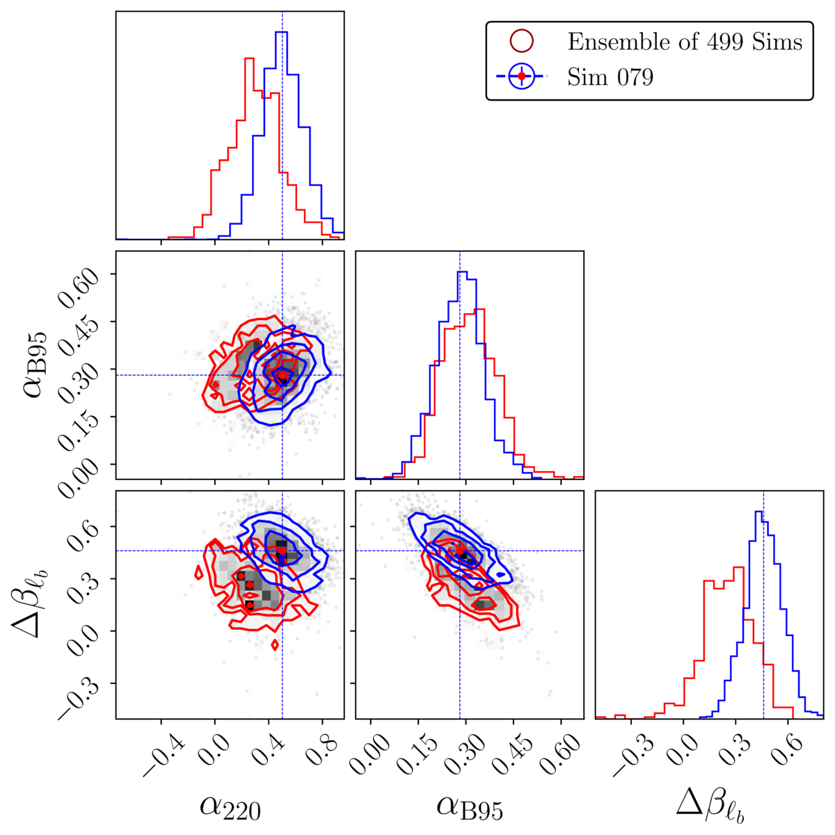
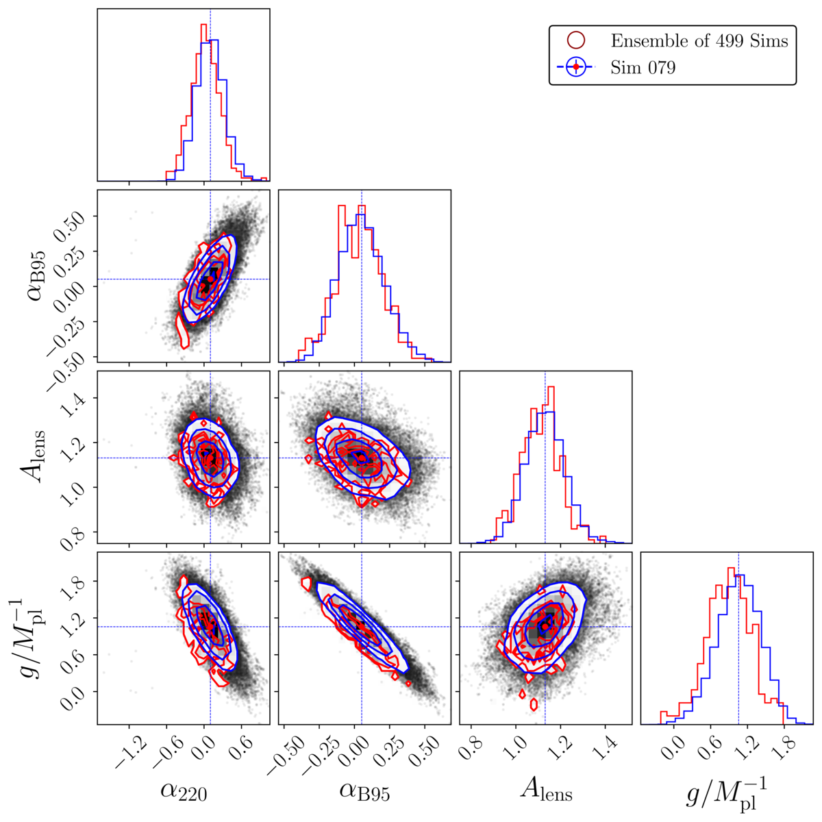
Figure S4: Contours show the posterior from a single representative realization (blue) compared to the distribution of best-fit peaks from 499 simulations (red) in the EDE set (“All with scaled BB”). The agreement between the single-realization width and the ensemble scatter indicates that the likelihood accurately estimates parameter uncertainties. Blue dashed lines mark the mean of Sim 79 realization's posterior, and the red dot marks its position on the ensemble contour. For visualization, the posterior is projected onto select parameters of interest; all other foreground and instrument parameters (see Tables S2 and S3) are marginalized over.
|
PDF / PNG |