-
BK-XX: Component-separated maps of polarized CMB and thermal dust emission using Planck and BICEP/Keck Observations through the 2018 Observing Season
The BICEP/Keck Collaboration, ApJ 999, 89, 2026
| Figures | Download Bundle | ||
|---|---|---|---|
| Maximum-likelihood \(\beta_d\) | 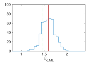 |
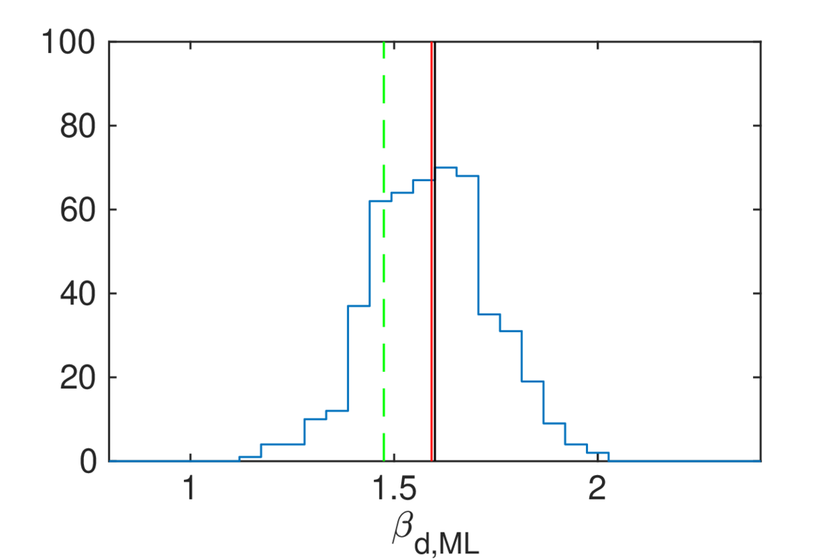
Figure 1: Histogram of the maximum likelihood values of the dust spectra index \(\beta_d\) obtained in the baseline BK18 auto-/cross-spectrum analysis. The black vertical line indicates the input value to the simulations, the (nearly conincident) red line indicates the mean of the recovered best-fit values, and the dashed green line marks the best-fit value of the real data. | PDF / PNG |
| BICEP observing matrix | 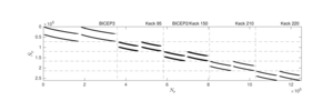 |
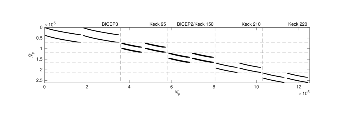
Figure 2: Plot of the non-zero matrix elements of the BICEP/Keck internal maps' observing matrices, i.e., the BICEP/Keck-specific block of the matrix \(\mathbf{R}\) used in this work. Applying a vector including beam-convolved Q & U maps to the right of this matrix results in a vector of filtered Q & U maps in the flat pixelization used in BK18. The top-left block corresponds to the BICEP3 map, while the following blocks along the diagonal contain the observing matrices for the Keck 95 GHz, BICEP2/Keck 150 GHz, Keck 210 GHz, and Keck 220 GHz channels. Within each block on the diagonal, the top row produces a BICEP/Keck Q map and the bottom row a BICEP/Keck U map from a vector of stacked Q & U maps. This part of the matrix contains about 5 billion non-zero elements and is the biggest computational challenge in this analysis. | PDF / PNG |
| Combination of maps | 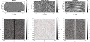 |
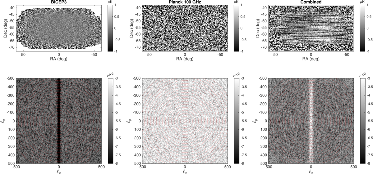
Figure 3: Q maps (top row) and the logarithmic (base 10) EE two-dimensional auto-power spectrum (bottom row) of one noise simulation for BICEP3 (left column), Planck HFI 100 GHz (middle column), and their combination (right column). The combination estimator corrects for filtering suppression at the map-level and hence boosts the noise compared to the filtered BICEP3 map and fills in modes from Planck for small \(\ell_x\). This is why the combined Q noise maps show strong horizontal stripes in the central BICEP3 map region. | PDF / PNG |
| Comparison of iterative solvers | 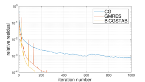 |
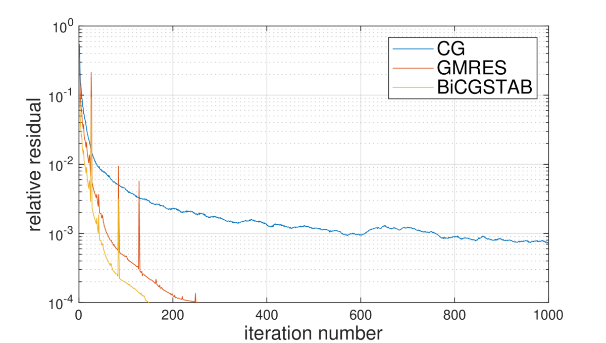
Figure 4: The relative residual \( || \mathbf{As} - \mathbf{b} || / || \mathbf{b} || \), where \( \mathbf{A} \equiv \mathbf{R}^T \hat{\mathbf{N}}_{B3}^{-1} \mathbf{R} + \hat{\mathbf{N}}_P^{-1}\) and \( \mathbf{b} = \mathbf{R}^T \hat{\mathbf{N}}_{B3}^{-1} \mathbf{d}_{B3} + \hat{\mathbf{N}}_P^{-1} \mathbf{d}_P\), for each iteration of the preconditioned iterative method. We test three different iterative solvers: the classic CG, GMRES, and Bi-CGSTAB. The spikes are due to numerical noise, which these iterative solvers are susceptible to. | PDF / PNG |
| Convergence for signal and/or noise simulations | 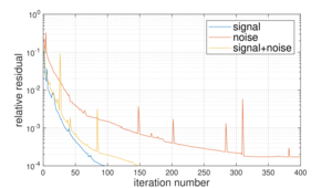 |
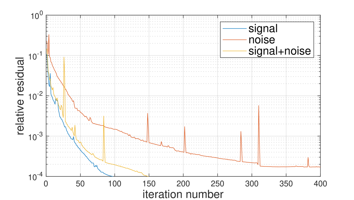
Figure 5: The relative residual as defined in Fig. 4 for each iteration of the (Bi-CGSTAB) preconditioned conjugate gradient method. We show the convergence performance for a signal-only, noise-only, and a signal-and-noise simulation. | PDF / PNG |
| Convergence for map combinations | 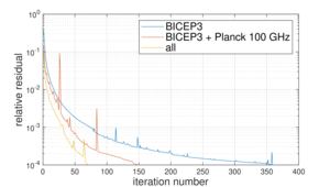 |
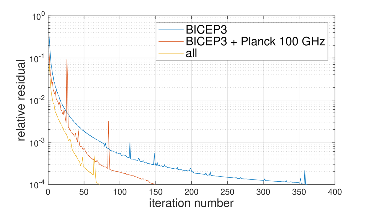
Figure 6: The relative residual as defined in the caption of Fig. 4 for each PCG iteration step. We show a comparison to solve for the frequency-map solution for BICEP3 and the BICEP3+Planck combination, as well as the CMB component map solution given all frequency maps as described in Sec. III. | PDF / PNG |
| Weight maps for CMB and dust | 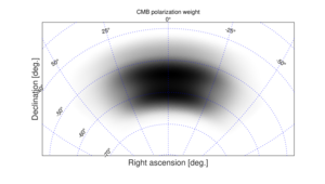 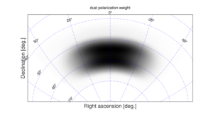 |
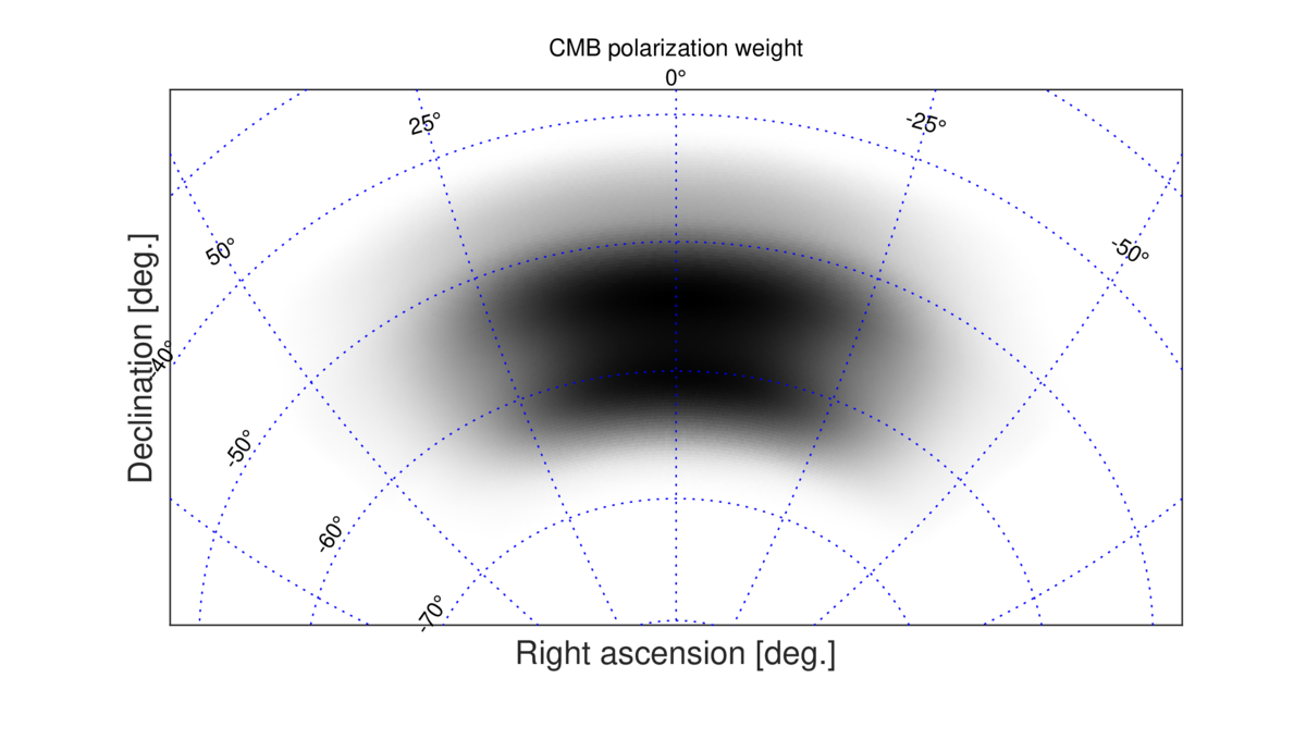
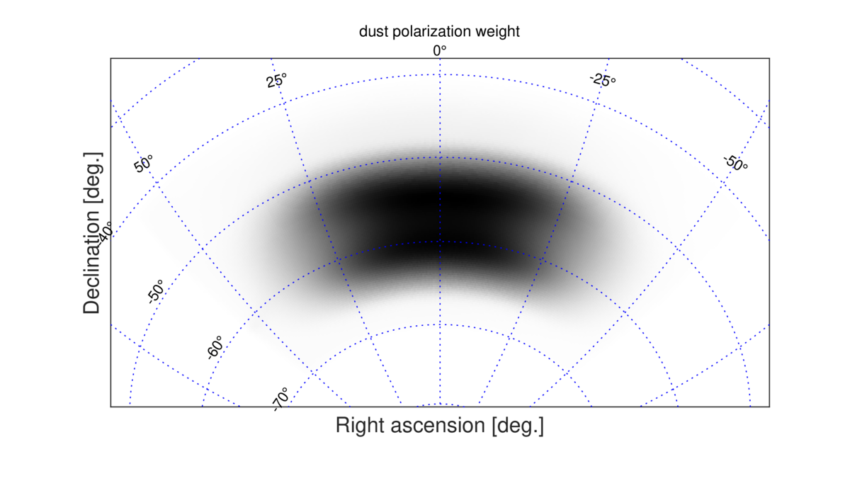
Figure 7: The polarization weight defined as the inverse arithmetic mean of the Q and U noise variance assuming white noise per pixel for the CMB component (top) and the dust component (bottom) in arbitrary units. Due to the extended coverage of BICEP3, the CMB extends above 50° in declination, while the dust component map is most sensitive in the BICEP2/Keck region. | PDFa PDFb / PNGa PNGb |
| Noise variance for CMB map | 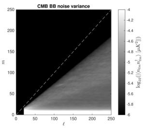 |
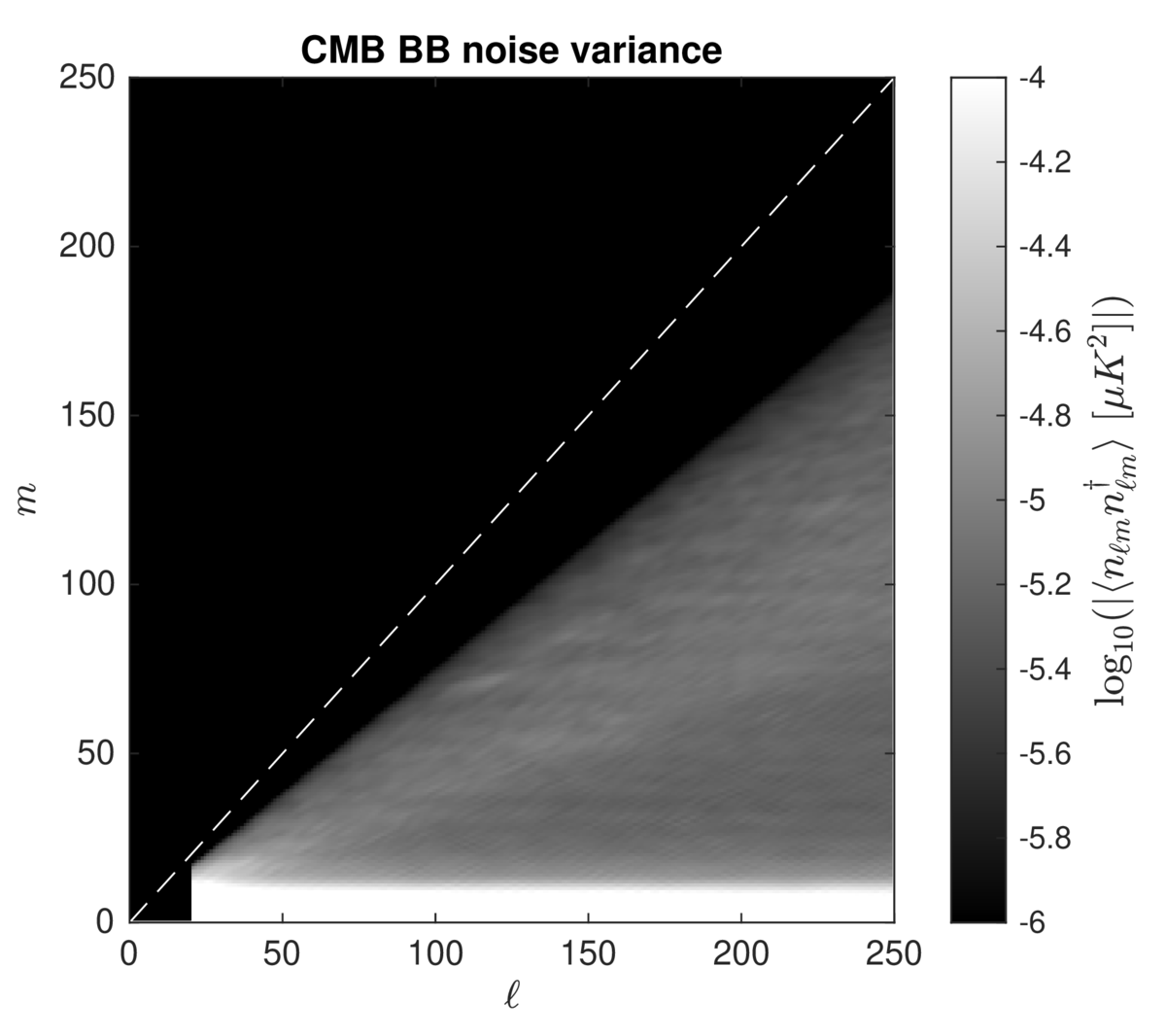
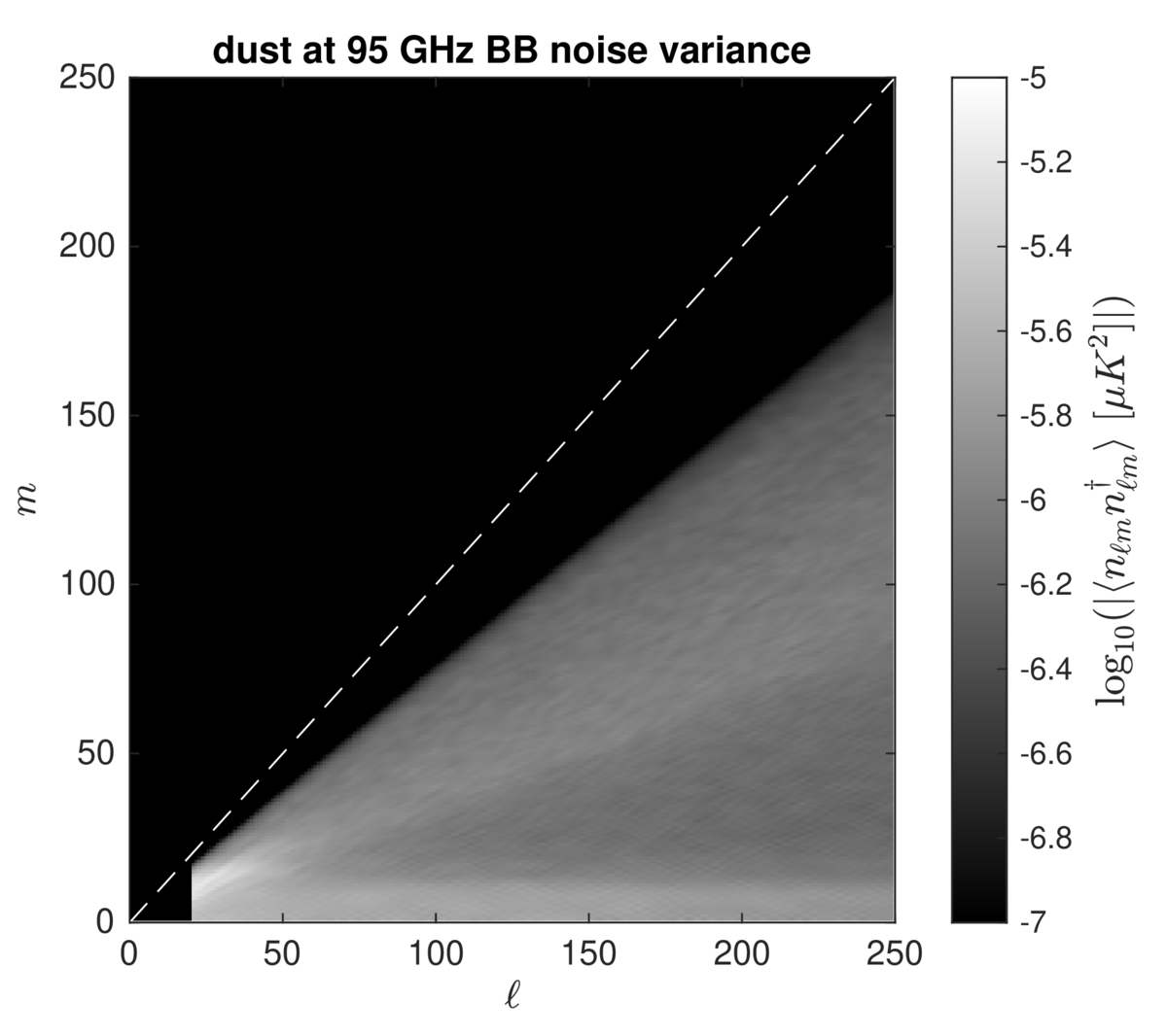
Figure 8: The noise variance per \( (\ell, m) \) mode of the CMB component map obtained by averaging over 499 noise-only simulations, after applying the corresponding map-level weight shown in Fig. 7 before computing harmonic coefficients. | PDF / PNG |
| Noise variance for dust map | 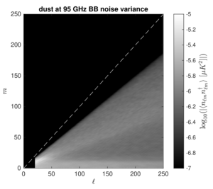 |
Figure 9: Same as Fig. 8 but for the dust component map scaled to 95 GHz. | PDF / PNG |
| CMB map and residuals | 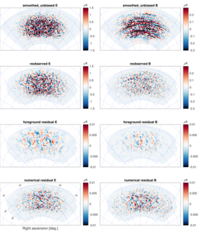 |
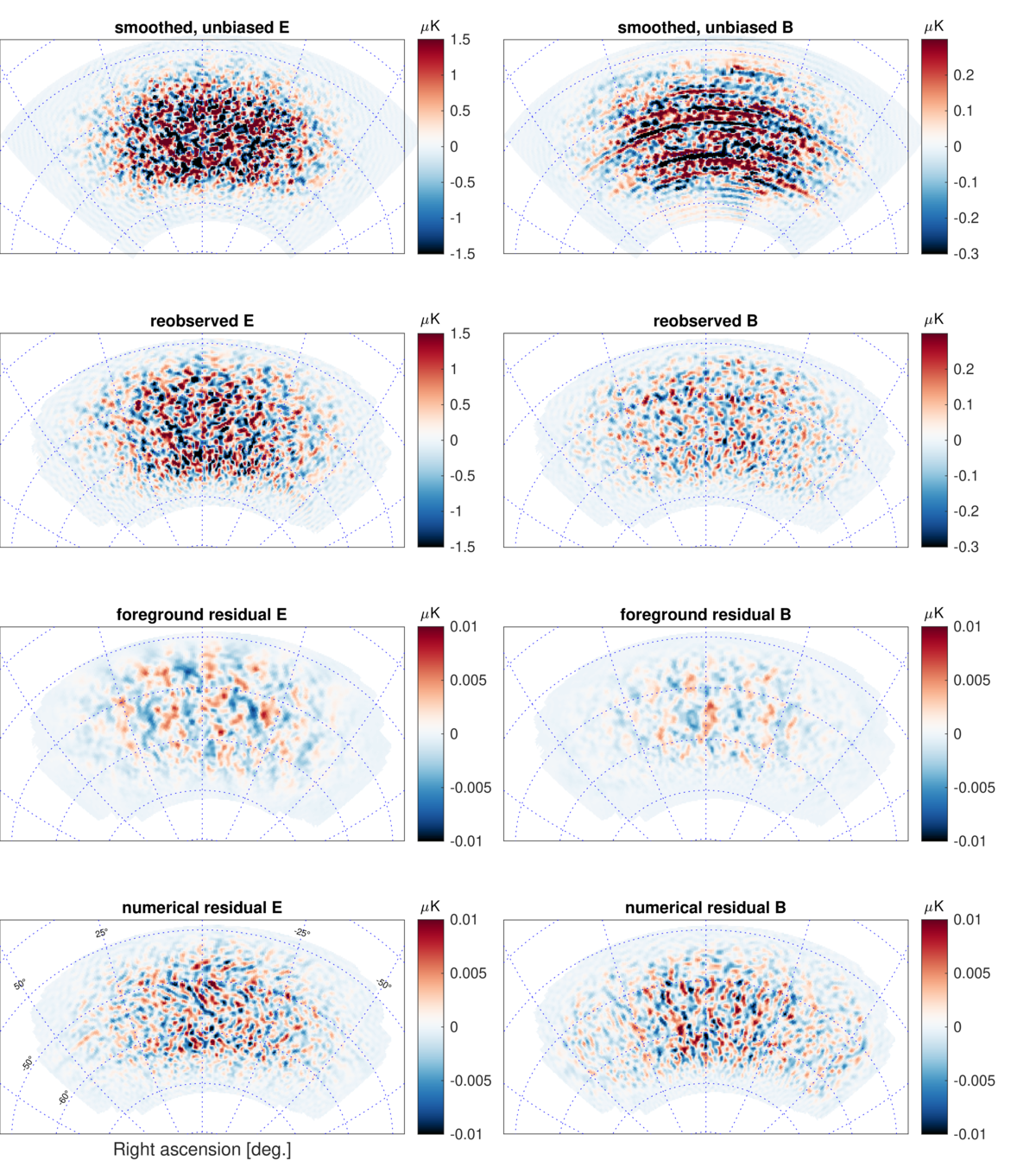
Figure 10: The CMB part of the component separated map estimator when run on a simulation, after apodization and B-mode purification. First row: The input is a simulated realization of lensed ΛCDM, galactic dust, and noise. The output has been convolved with a 20 arcmin Gaussian beam, multiplied with a pixel-space weighting and transformed into E and B-mode maps correcting for E-to-B-leakage effects from the masking. Second row: After applying the BICEP3 observing matrix and purifying using the corresponding purification matrix. Third row: Subtracting the corresponding CMB-and-noise-only simulation from the maps in the previous row reveals the residual from foreground. Given that the foreground simulations used here are isotropic and Gaussian, the residual is entirely caused by statistical fluctuation in the \(\beta_d\) fit. Fourth row: To get an estimate of the numerical residual, we subtract the corresponding BICEP3 CMB-only simulation from the CMB component map simulation. This contains effects from the small differences in the filtering done on actual timestreams versus what is incorporated into the observing matrix, and numerical errors coming from the spherical harmonic transforms and the iterative solution method applied to obtain the CMB component map estimate. Note the much reduced color range in rows three and four. |
PDF / PNG |
| CMB E and B-mode maps | 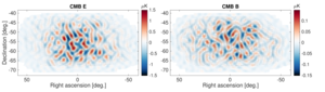 |
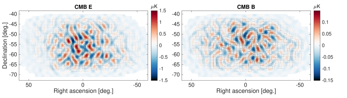
Figure 11: E-mode (left) and B-mode (right) maximum-likelihood maps of the CMB in CMB units, beam-convolved and filtered like a BICEP3 map at 95 GHz with an additional bandpass filter to degree angular scales (\(50 \lt \ell \lt 120\)). Note the differing color ranges; on the left, the E map is dominated by ΛCDM signal, whereas on the right the B map is approximately equal parts lensed-ΛCDM signal and noise. | PDF / PNG |
| Dust E and B-mode maps | 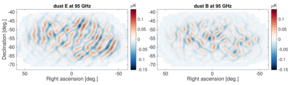 |
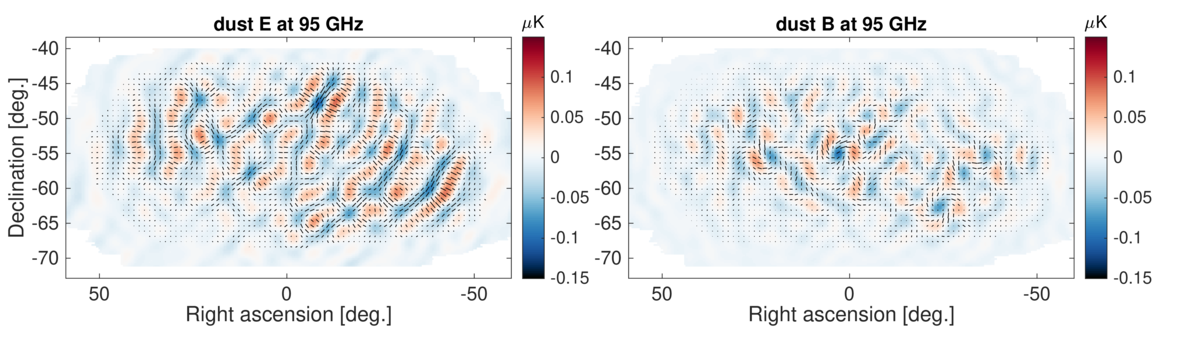
Figure 12: E-mode (left) and B-mode (right) maximum-likelihood maps of thermal dust in CMB units, beam-convolved and filtered like a BICEP3 map at 95 GHz with an additional bandpass filter to degree angular scales (\(50 \lt \ell \lt 120\)). The maps are apodized and B-modes are purified. The E-modes are visibly brighter than the B-modes. | PDF / PNG |
| Dust Q and U maps | 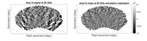 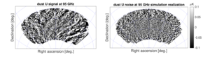 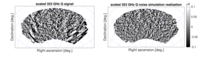 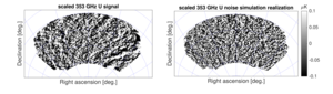 |
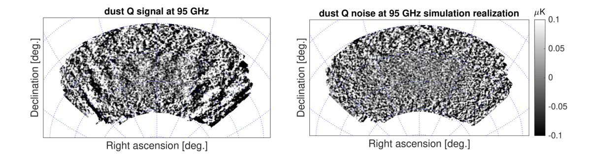
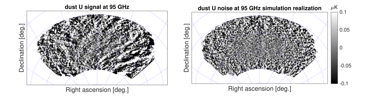
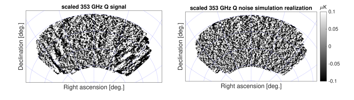
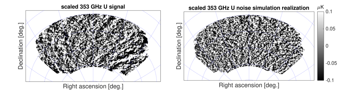
Figure 13: The first and second rows show the derived thermal dust component maps of this paper for Q and U signal (left), respectively, compared to a simulation of noise (right). The noise is lower in the central BICEP2/Keck region due to the high-frequency data from Keck. Structure in the dust polarization is apparent, particularly in the outer regions of the observing field. The third and fourth rows show equivalent Q and U maps for Planck 353 GHz data (left) and one noise simulation (right), scaled to 95 GHz using a modified blackbody (MBB) model with \(\beta_d = 1.5\). These Planck maps have been convolved to the same resolution as the derived component maps. All maps are reobserved with the BICEP3 observing matrix. | PDFa PDFb PDFc PDFd / PNGa PNGb PNGc PNGd |
| Comparison of pure-B estimators | 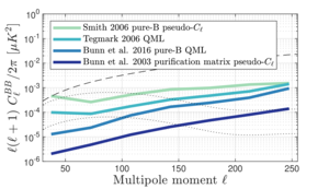 |
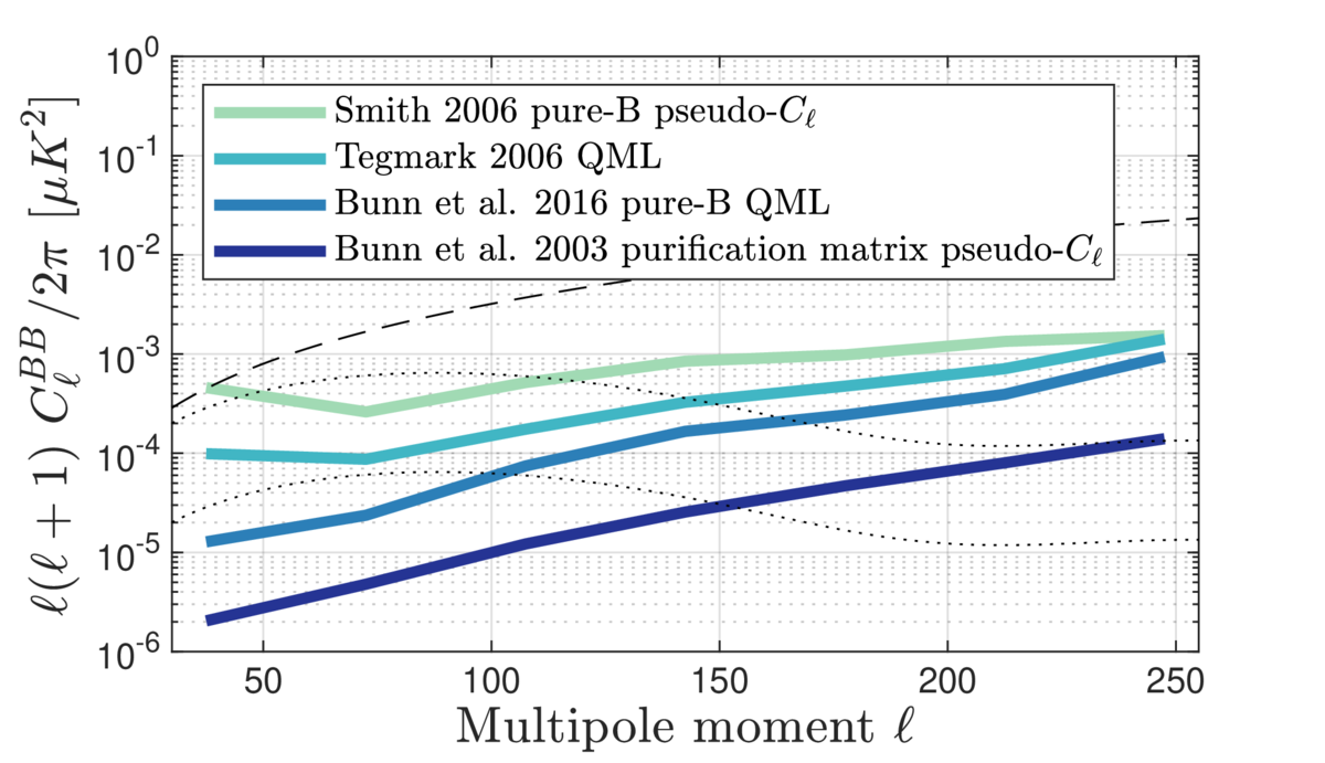
Figure 14: Comparing purification performance for different power spectrum estimators considered in this work: a simple pseudo-\(\mathcal{C}_\ell\) pure-B estimator of Ref. [26], optimal quadratic maximum-likelihood (QML) methods of Refs. [27] and [28], and a purification-matrix-based method described in Ref. [31] and used in previous BICEP/Keck analyses. The dashed line corresponds to the lensed-B power of our baseline ΛCDM model, while the dotted lines correspond to a primordial gravitational wave signal of \(r = 10^{-2}\) and \(r = 10^{-3}\). | PDF / PNG |
| Noise power and effective sky fraction | 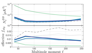 |
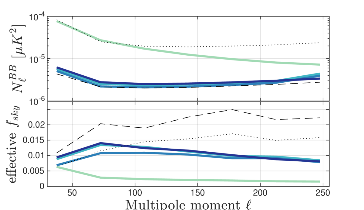
Figure 15: First row: The noise spectra for the different power-spectrum estimators run on the CMB component map. Colors are the same as in Fig. 14. The BICEP3 95 GHz noise and the Keck 220 GHz noise are shown in the black dashed and dotted lines, respectively. The spectra are shown after correction for the filtering of signal which occurs due to the beam roll-off, timestream filtering, and B-mode purification. (Note that no \(\ell^2\) scaling is applied.) Second row: The effective sky fraction as calculated from the ratio of the mean noise realization bandpowers to their fluctuation \( f_\mathrm{sky}(\ell) = \frac{1}{2\ell\Delta\ell} \left( \frac{\sqrt{2} \bar{N}_b}{\sigma(N_b)} \right)^2 \), i.e. the observed number of B-mode degrees of freedom divided by the nominal full-sky number. | PDF / PNG |
| Suppression factor ratio | 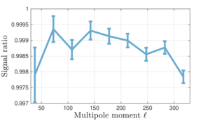 |
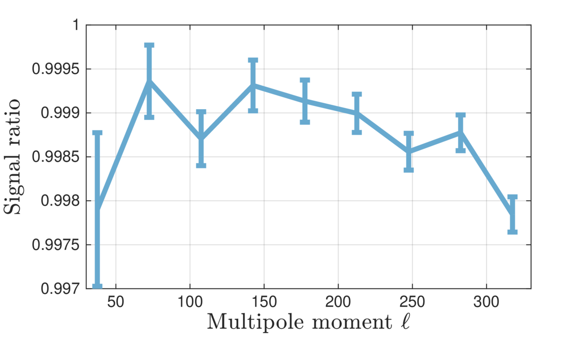
Figure 16: Suppression factor of the CMB component map computed as the ratio between the mean of power spectra of 499 signal-only simulations and the expectation for each bandpower. Error bars show the standard error of this mean. | PDF / PNG |
| Foreground residual from Gaussian dust simulations | 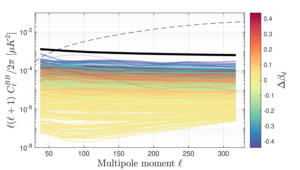 |
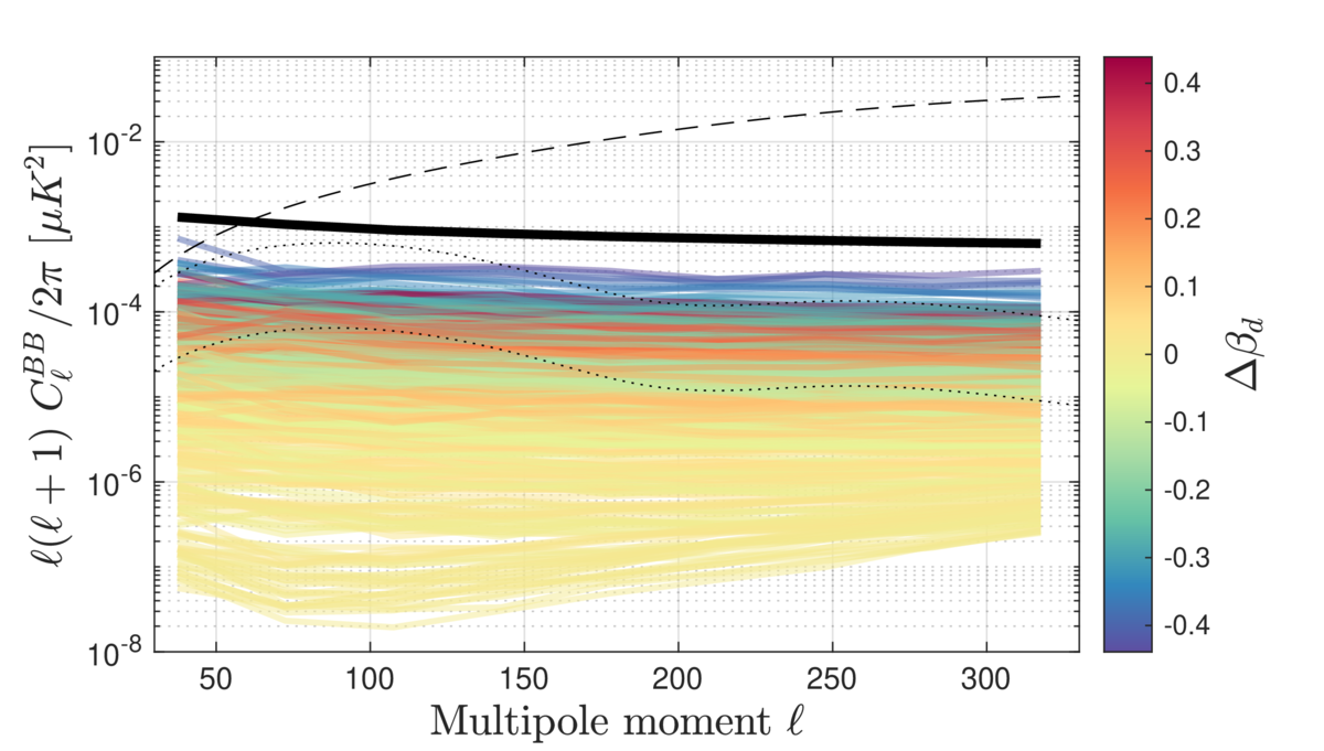
Figure 17: Foreground residual in the CMB component B-mode auto-power spectrum for 499 Gaussian-dust-only simulations. The color of the lines show the deviation of the respective best-fit value of \(\beta_d\) for the specific realization from the simulation input of \(\beta_d^\mathrm{true} = 1.6\). The thick solid black line indicates the dust level at 95 GHz, without any foreground cleaning, as measured in Ref. [3]. The dashed line corresponds to the lensed-B power of our baseline ΛCDM model while the dotted lines correspond to a primordial gravitational wave signal of \(r = 10^{-2}\) and \(r = 10^{-3}\). | PDF / PNG |
| Foreground residual from alternate dust simulations | 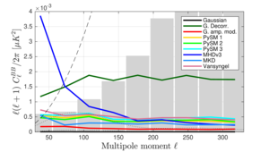 |
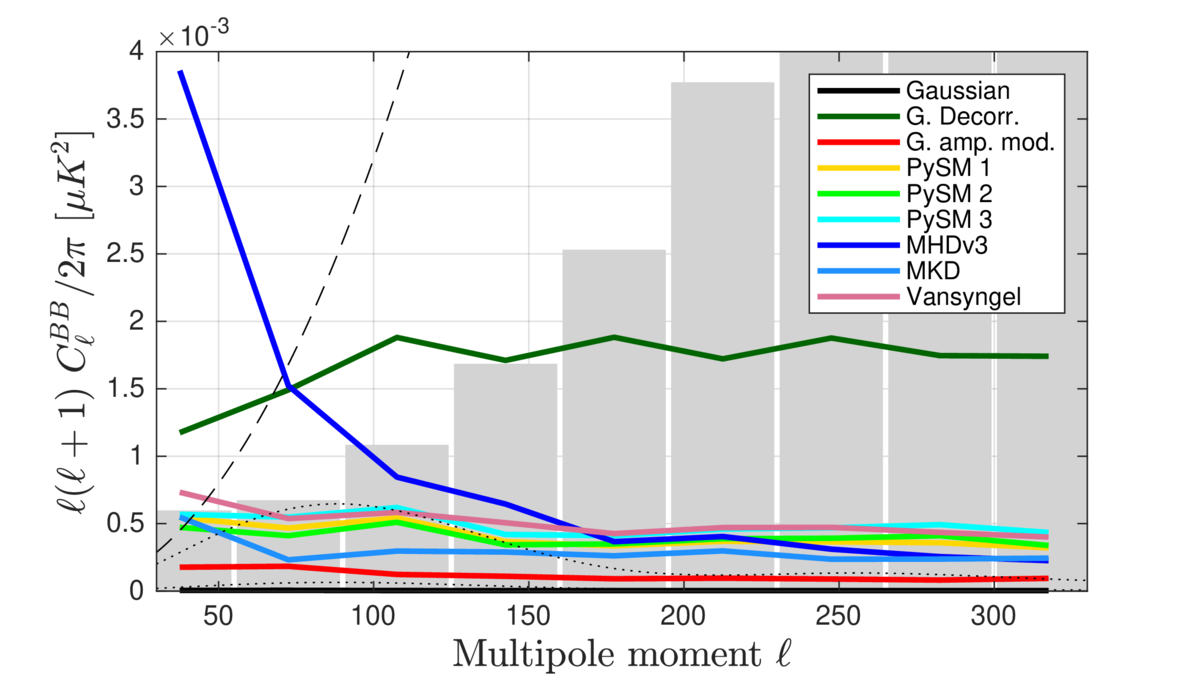
Figure 18: Systematic bias from one realization of the Gaussian and the alternate dust models as described in Refs. [3, 13] and Sec. VII B. The gray bars represent the standard deviation of ΛCDM+dust+noise simulations in each bandpower. Most models lead to residuals smaller than this scatter representing cosmic variance. The dashed line corresponds to the lensed-B power of our baseline ΛCDM model. | PDF / PNG |
| CMB and dust bandpowers | 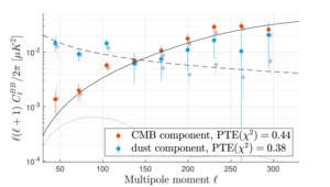 |
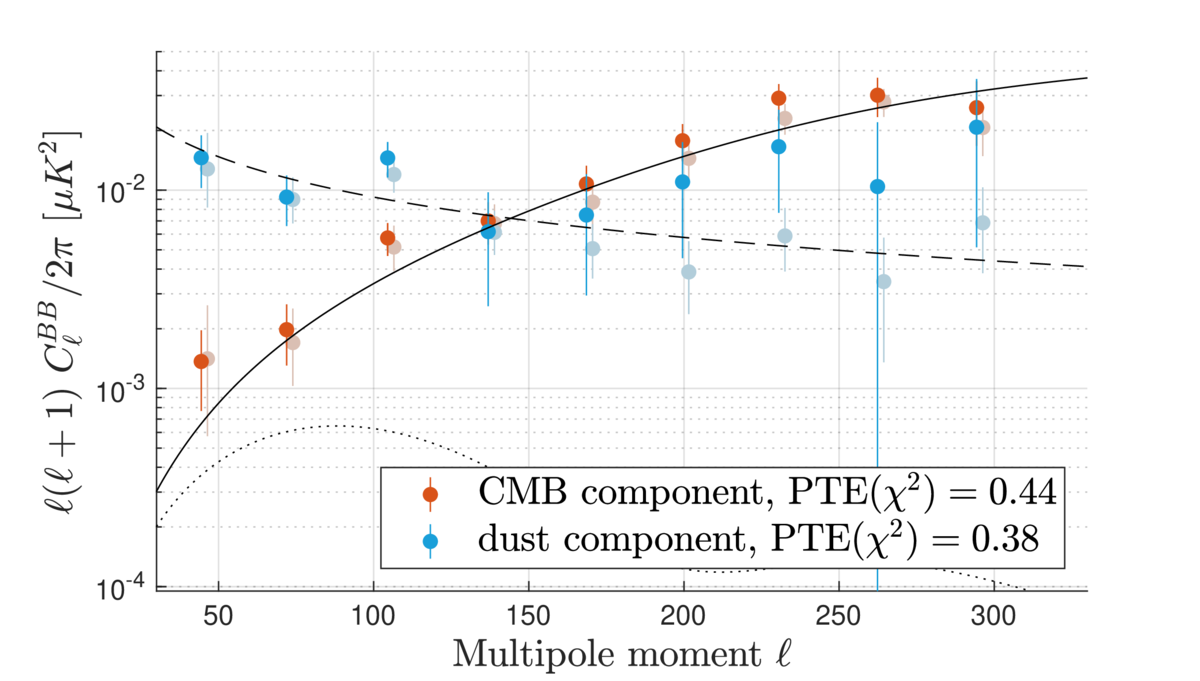
Figure 19: Real-data bandpowers of the CMB (orange points) and dust (blue points) component maps. The solid black line is the fiducial ΛCDM B-mode power spectrum from CMB lensing, the dotted black line is the primordial B-mode power spectrum for \(r = 10^{-2}\), and the dashed black line corresponds to the best-fit dust model of Ref. [3] at 150 GHz. The faint points are derived using the cross-frequency likelihood method, where results represent a full MCMC sampling of the posterior within each individual bandpower bin; these are equivalent to Fig. 16 of BK18 but with marginalization over synchrotron parameters removed. The \(\chi^2\) PTE values for the CMB and dust components, comparing the data bandpowers to the ΛCDM and best-fit dust models, are 0.44 and 0.38, respectively. | PDF / PNG |
| Correlation with BK18 baseline analysis method | 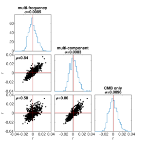 |
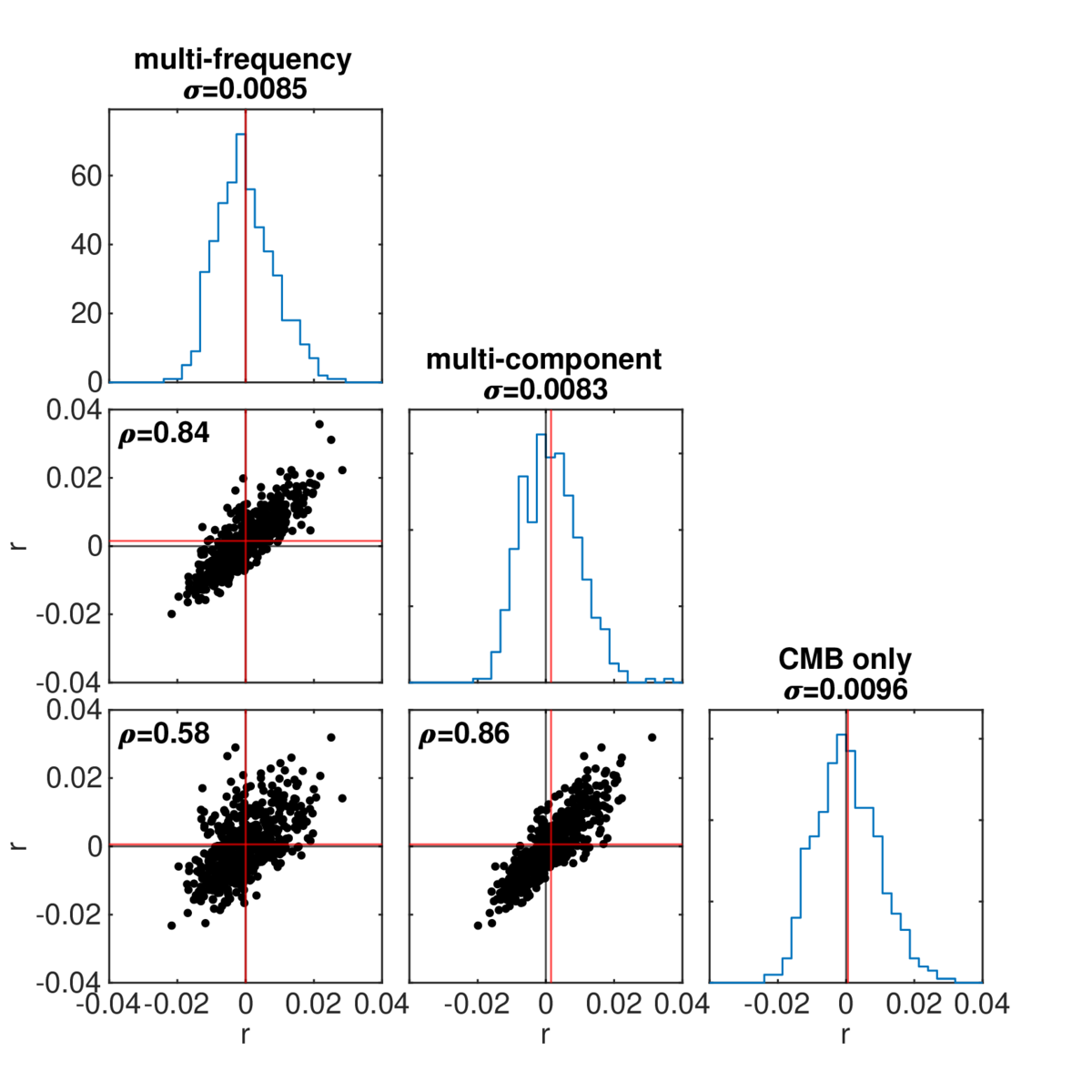
Figure 20: Histograms and 2D scatter plots between best-fit \(r\) values obtained with the multi-frequency-spectrum-based method of Ref. [3] (with the modification of fixing the synchrotron component in the model and aligning the selected frequency bands with those used in this paper) and the multicomponent-spectrum-based method presented in this paper, either including or excluding the dust component map in the power spectrum computation. Black vertical and horiontal lines show the simulation input of \(r = 0\), while the corresponding red lines show the distribution mean. The distribution standard deviations are shown in the respective histogram's title. The Pearson correlation coefficient, \(\rho\), ranges from 58% to 86%. | PDF / PNG |
History
- 2026-07-15: Posted BK-XX: Component-separated maps of polarized CMB and thermal dust emission using Planck and BICEP/Keck Observations through the 2018 Observing Season figures.