| A schematic of the BICEP2 optical chain |
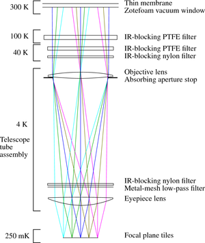 |
Figure 1:
A schematic of the BICEP2 optical chain with each optical element labeled.
The relative position of the lenses and focal plane is to scale. The Keck Array optical chain is identical
except that the IR-blocking
filters in front of the objective lens are all on the 50 K stage in the Keck Array and the positions of the
metal-mesh low pass filter and 4 K nylon filter are reversed.
|
PDF / PNG |
| BICEP2 and Keck Array |
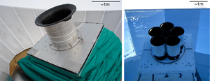 |
Figure 2:
A picture of BICEP2 (left) and the Keck Array (right) from the outside. The forebaffles and the reflective ground shield
are visible.
|
PDF / PNG |
| Simulated far-field beam pattern |
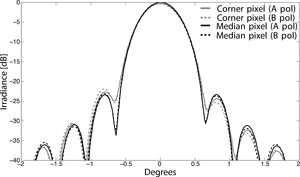 |
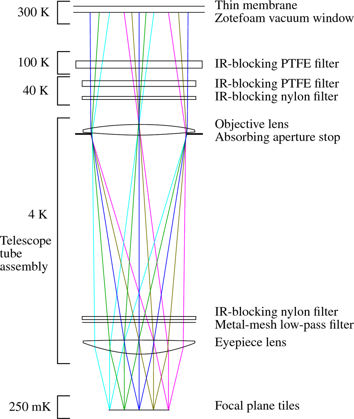
Figure 3:
Simulated far-field beam pattern for orthogonally polarized A and B beams, for both median-radius and
corner pixels in the focal plane. Beams share the same peak normalization.
|
PDF / PNG |
| A measurement of the near-field beam pattern |
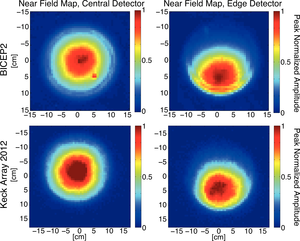 |
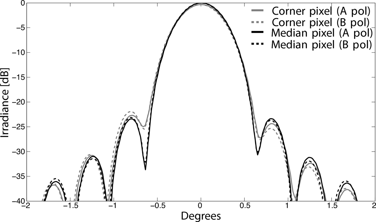
Figure 4: A measurement of the near-field beam pattern for two example channels
in BICEP2 and the Keck Array during 2012. Left: A detector near the center of a tile in the
focal plane. Right: A detector near the edge of the
focal plane, showing significant truncation by the aperture (worst case). This truncation leads to
moderate ellipticity in the far field.
The sharp feature seen for the center pixel in BICEP2 is from a
reflection off of the 4 K nylon filter, and is diffusely coupled to the sky.
|
PDF / PNG |
| Example Keck Array near field beam mismatch |
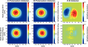 |
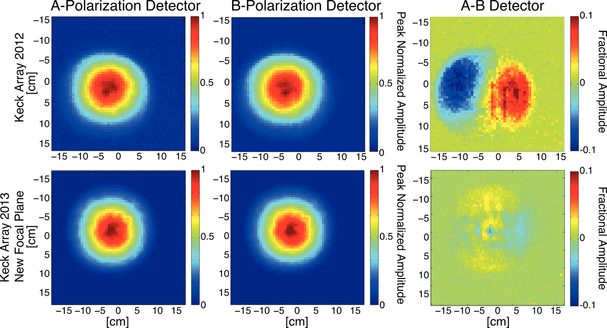
Figure 5:
An example Keck Array detector pair that shows beam mismatch in the near field. Left: The optical response of
an A polarization detector in a typical detector pair.
Center: The optical response of the co-located B polarization
detector. Right: The fractional difference between the A and B optical response. The top panels show a typical
detector pair from a focal plane
in 2012, and the bottom panels show a typical detector pair from the new focal plane installed in 2013
with dramatically reduced
differential pointing.
|
PDF / PNG |
| The setup for measuring far-field beam patterns |
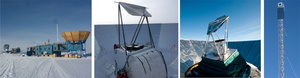 |
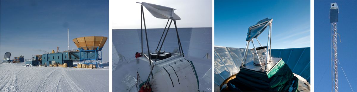
Figure 6: The setup for measuring far-field beam patterns of BICEP2 and Keck Array
detectors in situ
at the South Pole. A chopped thermal source broadcasts from a mast on MAPO or DSL,
and a large aluminum honeycomb mirror
is installed to redirect the beams of BICEP2 and the Keck Array to the source. Left: DSL (far) and MAPO (near),
home of BICEP2 and the Keck Array. Both masts are up and are being used for beam mapping. Center Left:
The large mirror installed for beam mapping on the Keck Array. Center Right: The smaller
mirror installed for beam mapping
on BICEP2. Right: A close up of a microwave source mounted on the mast.
|
PDF / PNG |
| Far-field response maps |
 |
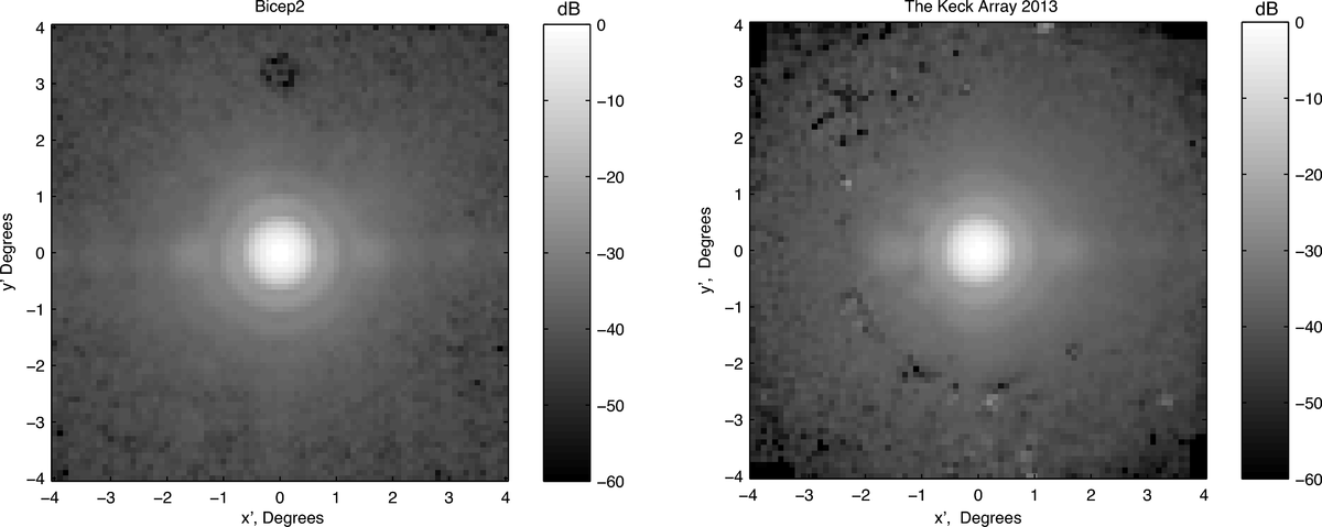
Figure 7: Left: A map of the BICEP2 far-field response made with a thermal
source, centered, rotated,
and co-added over all operational channels from 2012 data. Right: A map of
the Keck Array far-field response made with a
thermal source, centered, rotated,
and co-added over all operational channels for all 2013 Keck Array receivers.
The color scale is logarithmic with decades marked in dB.
The measured main beam shape and Airy ring structure are well-matched by simulations. Cross-talk features
are evident, 1.5° to the right and left of the main beam.
The feature 3° above the main beam in the BICEP2 is also due to crosstalk.
|
PDF / PNG |
| Azimuthally averaged beam profiles |
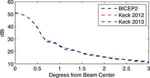 |
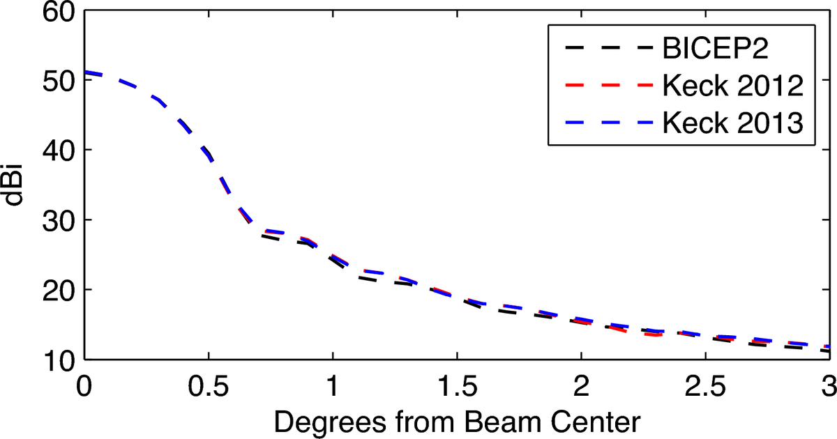
Figure 8: Azimuthally averaged beam profiles for BICEP2 and
the Keck Array for 2012 and 2013, co-added over all operational channels.
|
PDF / PNG |
| Example far-field beam patterns |
 |
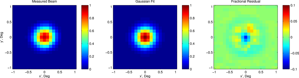
Figure 9:
Left: Example measured far-field beam pattern from BICEP2, linear scale. Middle: Gaussian fit
to measured beam pattern. Right: Fractional
residual after subtracting the Gaussian fit in the middle panel. The residual represents
the portion of the beam that is not mitigated with the deprojection technique.
Note: The right-hand panel has a different
color scale than the left two panels.
|
PDF / PNG |
| Per-detector beam ellipticity for BICEP2 |
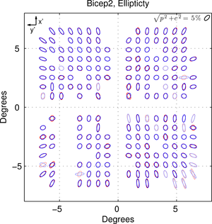 |
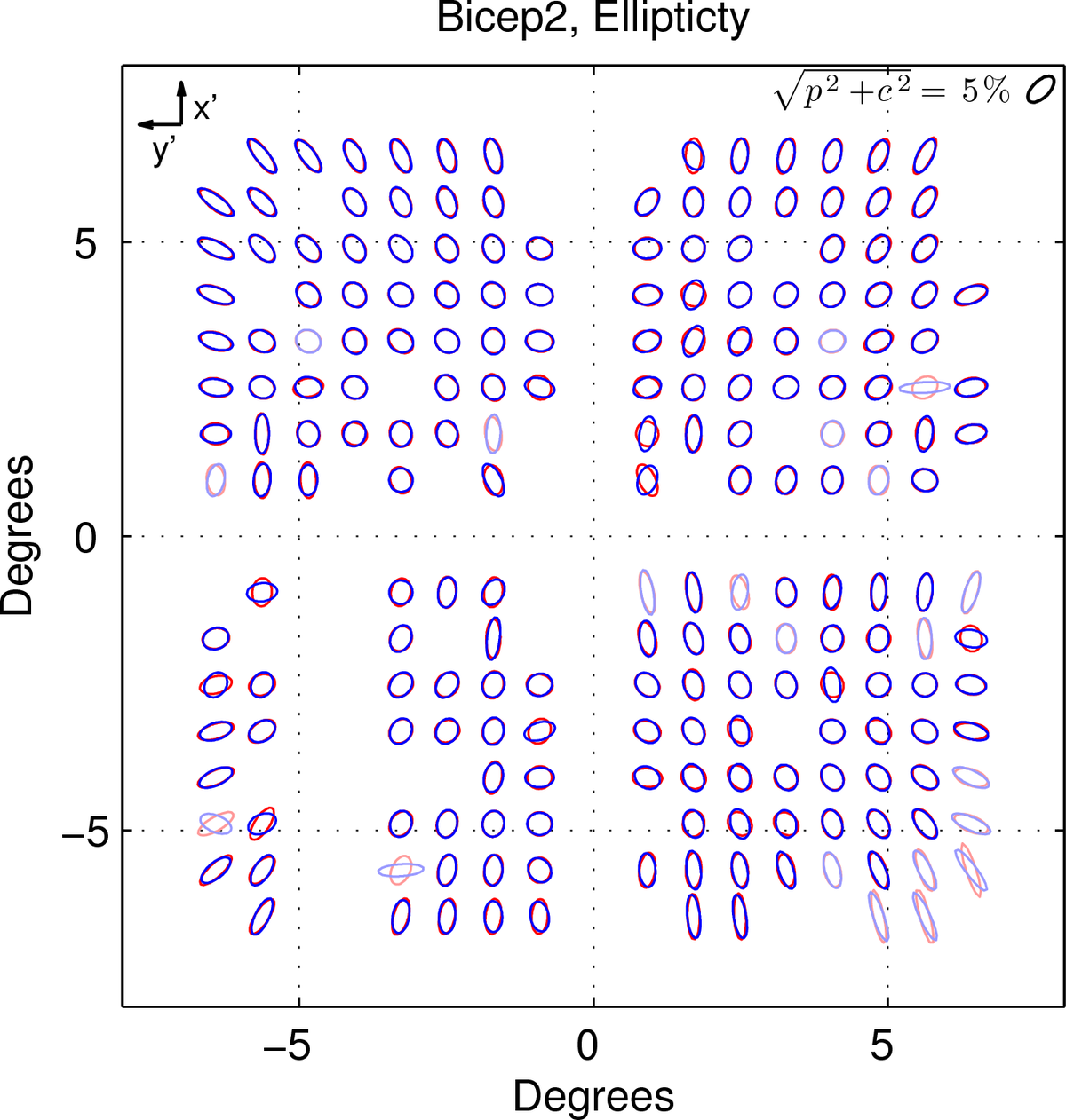
Figure 10:
Per-detector beam ellipticity for BICEP2 as projected onto the sky.
The ellipticity for each detector has been exaggerated for visibility, as shown in the legend.
A and B beams are
shown in red and blue, respectively, and light colors show detectors that are not used in analysis.
|
PDF / PNG |
| Per-detector beam ellipticity for the Keck Array |
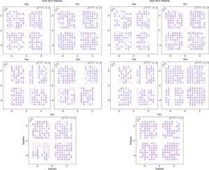 |
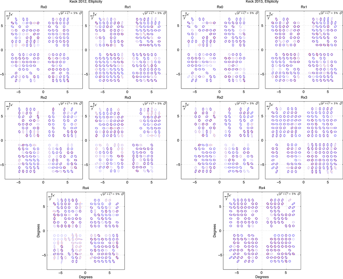
Figure 11:
Per-detector beam ellipticity for the Keck Array 2012 and 2013 configurations as projected onto the sky.
The ellipticity for each detector has been exaggerated for visibility, as shown in the legend.
A and B beams are
shown in red and blue, respectively, and light colors show detectors that are not used in analysis.
Detectors in Receivers 0, 2,
and three of the four tiles on Receiver 1 are the same between 2012 and 2013, and the correlation
between years for those receivers is evident.
|
PDF / PNG |
| Per-detector beam width |
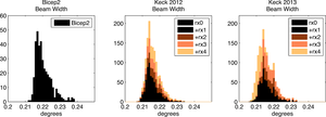 |
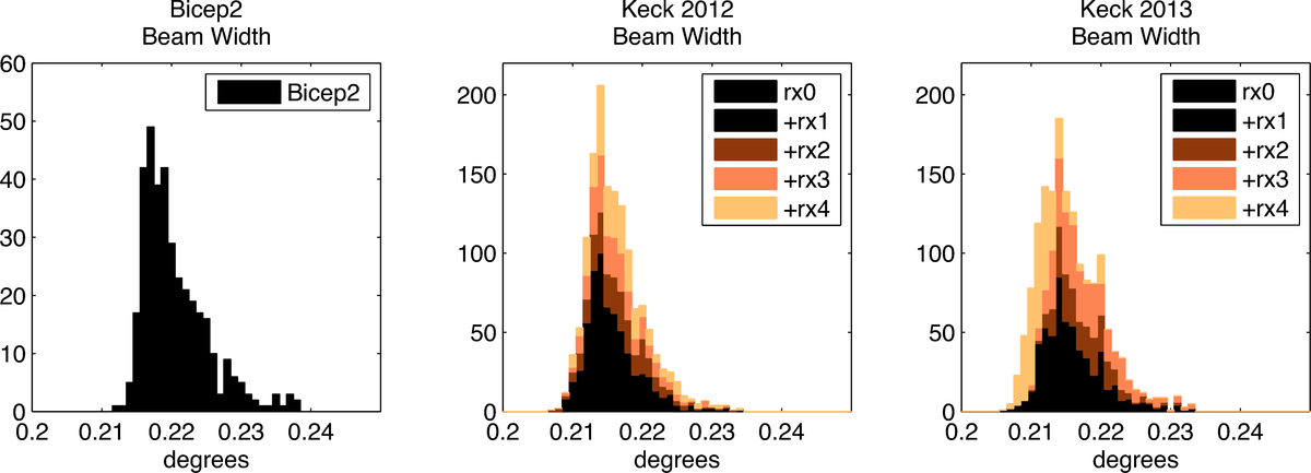
Figure 12:
Per-detector beam width (σ) measurements for BICEP2 (left-hand panel) and the Keck Array 2012 (middle panel)
and 2013 (right-hand panel).
|
PDF / PNG |
| Differential pointing measured for BICEP2 |
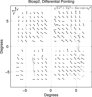 |
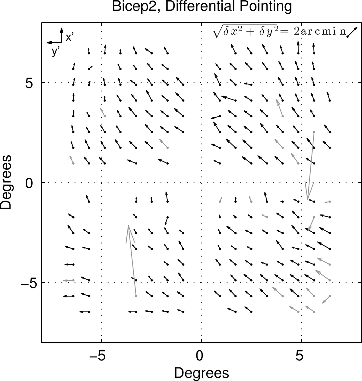
Figure 13: The differential pointing measured between orthogonally polarized,
co-located detector pairs, plotted in a focal plane layout for BICEP2.
Arrows point from the A detector location to the B detector location, and the length of the arrows
corresponds to the degree of mismatch multiplied by a factor of 20 for plotting. Detector pairs with
grey arrows are not used in analysis.
|
PDF / PNG |
| Differential pointing measured for Keck Array |
 |
Figure 14: The differential pointing measured between orthogonally polarized,
co-located detector pairs, plotted in a focal plane layout for the Keck Array in its 2012 and 2013 configurations.
Arrows point from the A detector location to the B detector location, and the length of the arrows
corresponds to the degree of mismatch multiplied by a factor of 20 for plotting. Detector pairs with
grey arrows are not used in analysis. Detectors in Receivers 0, 2,
and three of the four tiles on Receiver 1 are the same between 2012 and 2013, and the correlation
between years for those receivers is evident. Receiver 4 received a new
focal plane in 2013 with reduced near-field differential pointing.
|
PDF / PNG |
| Differential ellipticity measured for BICEP2 |
 |
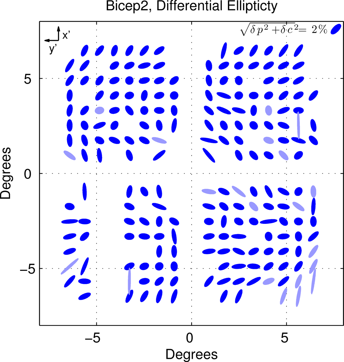
Figure 15: The differential ellipticity measured between orthogonally polarized,
co-located detector pairs, plotted in a focal plane layout for BICEP2. The
major axes of the ellipses are proportional to √(δ p2 + δ c2), a measure of the magnitude of
the differential ellipticity. A large fraction of
detectors have beams whose ellipticity is well matched. Light colored detector pairs are not used in analysis.
The differential ellipticity for each detector pair has been exaggerated for visibility, as shown in the legend.
|
PDF / PNG |
| Differential ellipticity measured for Keck Array |
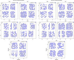 |
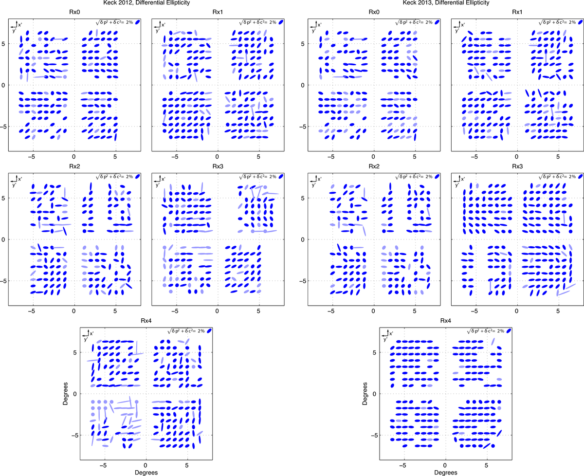
Figure 16: The differential ellipticity measured between co-located detector pairs, plotted
in a focal plane layout for the Keck Array 2012 and 2013. The
major axes of the ellipses are proportional to √(δ p2 + δ c2), a measure of the magnitude of
the differential ellipticity.
Light colored detector pairs are not used in analysis. The differential ellipticity for each
detector pair has been exaggerated for visibility, as shown in the legend.
Detectors in Receivers 0, 2,
and three of the four tiles on Receiver 1 are the same between 2012 and 2013, and the correlation
between years for those receivers is evident.
|
PDF / PNG |
| Measured differential beam width |
 |
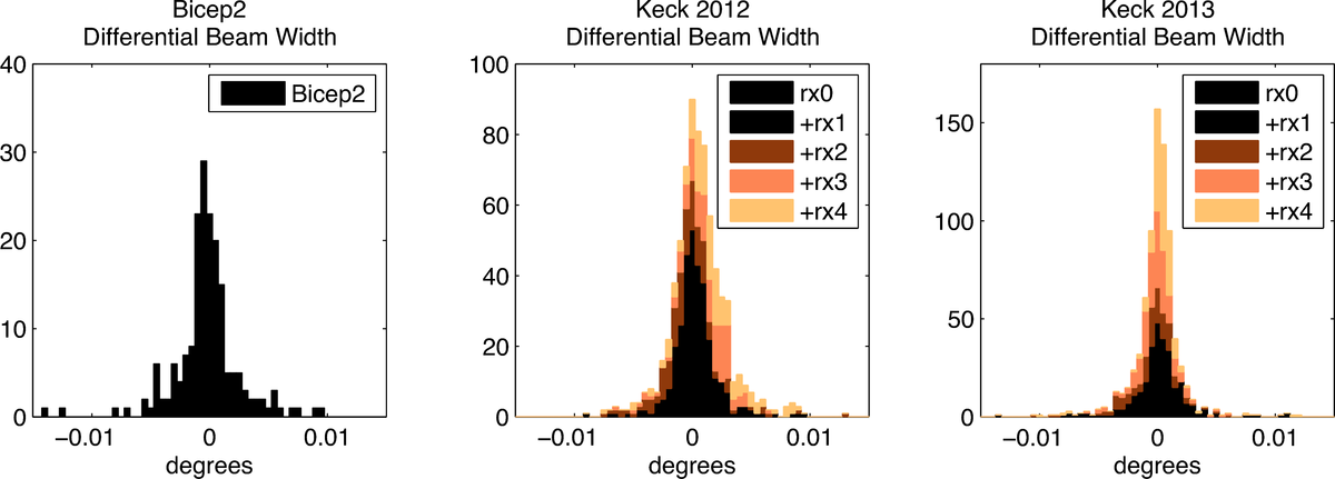
Figure 17: The measured differential beam width between orthogonally polarized,
co-located detector pairs for BICEP2 (left-hand panel) and the Keck Array 2012 (middle panel) and 2013 (right-hand panel).
|
PDF / PNG |
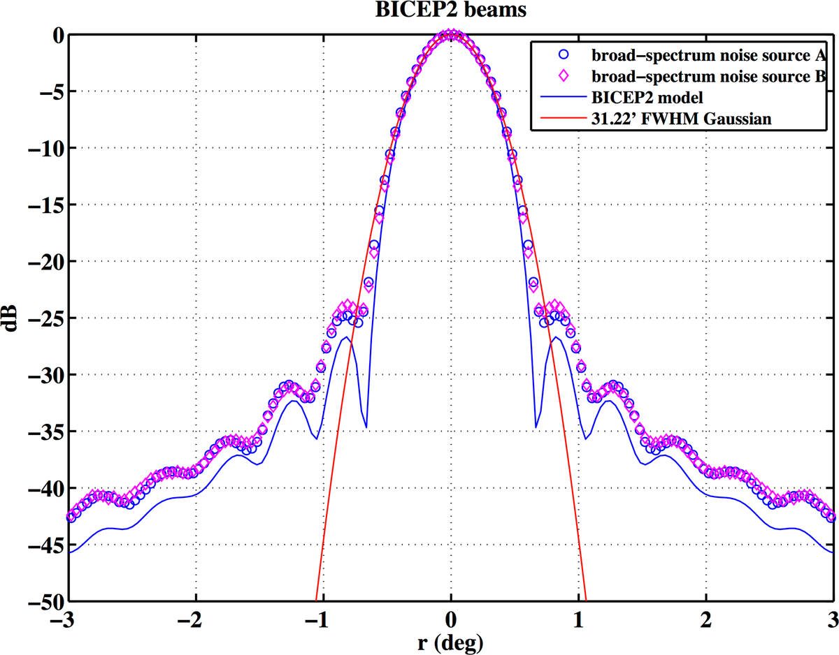
| Cross section of typical BICEP2 beams |
 |
Figure 18: Cross section of typical BICEP2 beams compared with Zemax physical optics
simulations and
a Gaussian fit. The agreement between the measured beams and the simulation is good, and the data are well-fit by
a Gaussian model near the peak.
|
PDF / PNG |
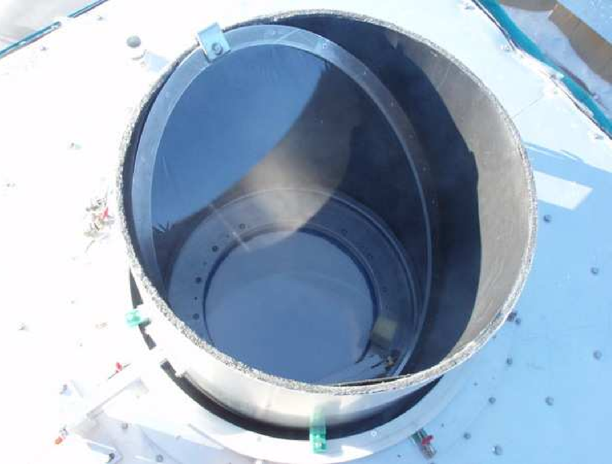
| Dielectric sheet calibrator |
 |
Figure 19: A picture of the dielectric sheet calibrator installed on the BICEP1 telescope. We
used this calibrator to measure the polarization angle and cross-polar response of BICEP2 as well.
|
PDF / PNG |
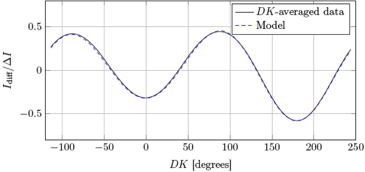
| The dielectric sheet calibrator pair-difference amplitude for a
typical pair of detectors |
 |
Figure 20: The dielectric sheet calibrator pair-difference amplitude for a
typical pair of detectors
in BICEP2 (Idiff),
normalized by the difference in temperature between the warm absorber and the sky (Δ I),
plotted as a function of boresight rotation angle (DK).
The fitted model is also plotted.
|
PDF / PNG |
| Rotating polarized amplified thermal broad-spectrum noise source |
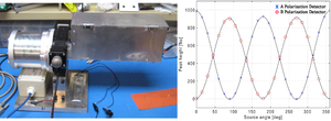 |
Figure 21: Left: The rotating polarized amplified thermal broad-spectrum noise source
used for polarization characterization. Right: Polarization modulation vs. source angle of an example
detector pair from BICEP2, measured
using the rotating polarized source.
|
PDF / PNG |
| Stokes T, Q, and U beam maps |
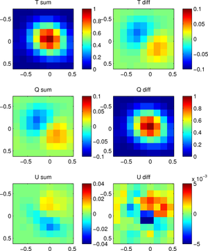 |
Figure 22:
The Stokes T, Q, and U beam maps (BT, BQ, and BU)
for a single typical pixel in BICEP2 from RPS measurements, smoothed
with a 0.1° Gaussian kernel.
The left column shows the response of the sum of the detectors in a pair; the right column shows the
pair difference response. The
pair difference BT and pair sum BQ both
show the differential pointing present in BICEP2.
An ideal instrument would have no U response.
Only the pair difference beams are relevant to BICEP2 polarization analysis.
The small (≲0.8%) features in the pair difference BU
cause a negligible amount of E-to-B leakage.
The larger feature in the pair sum BU beam would cause polarization to temperature
leakage, which is harmless.
Note that the color scales are not uniform across panels.
|
PDF / PNG |
| Differential beam templates |
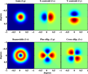 |
Figure 23: Differential beam templates resulting in mismatch in (a) responsivity
(b) x-position (c) y-position (d) beam width (e)
ellipticity in plus orientation (f) ellipticity in cross orientation. In the limit of small differential
parameters, a differenced beam
pattern constructed from the difference of two elliptical Gaussians
can be represented as a linear combination of each of these templates.
|
PDF / PNG |
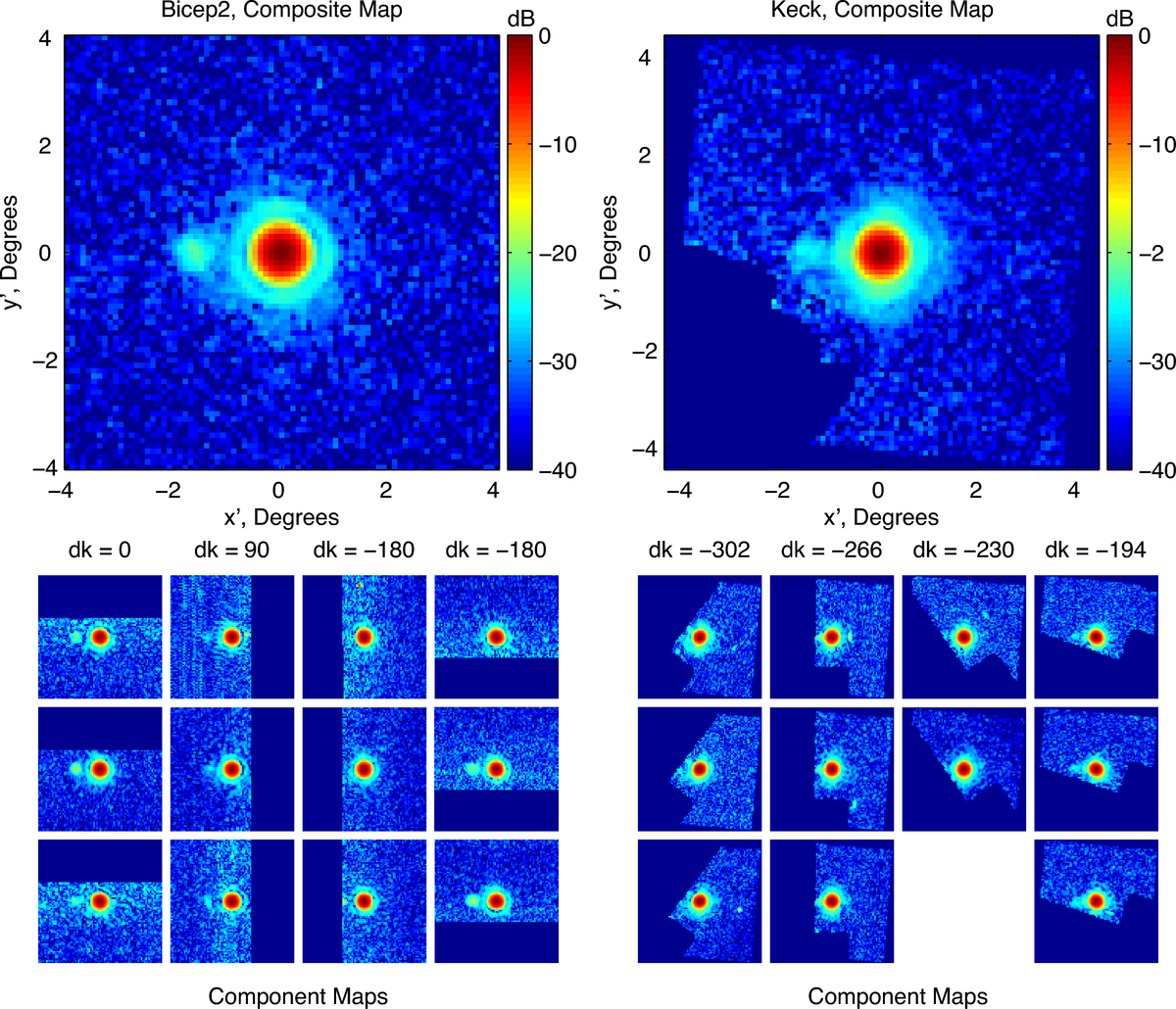
| Example composite beam maps |
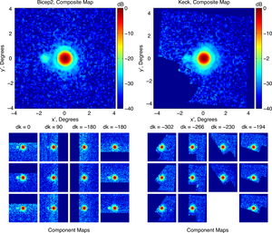 |
Figure 24:
Left: An example composite beam map for a BICEP2 detector using twelve beam maps.
Right: An example composite beam map
for a Keck Array detector using eleven beam maps. The maps are rotated to account
for the boresight rotation angle and then added. The color scale is logarithmic with decades marked in dB.
|
PDF / PNG |
| Comparison of deprojection coefficients |
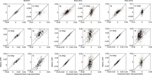 |
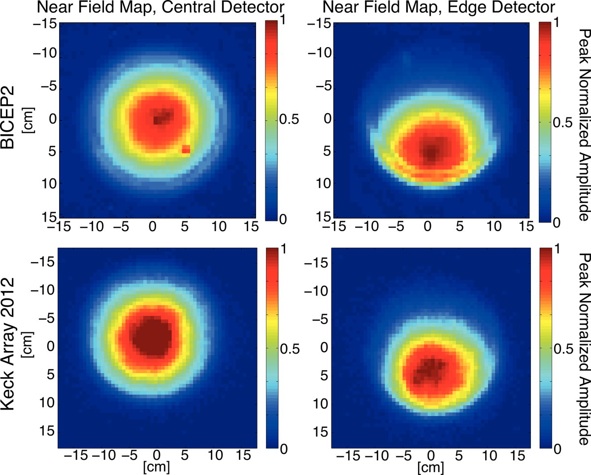
Figure 25: A comparison of the deprojection coefficients recovered using our
CMB observation data to the measured beam parameters from beam maps for BICEP2 and
the Keck Array 2012 and 2013.
We observe a strong correlation for differential pointing and differential ellipticity for BICEP2, and a
strong correlation for differential pointing in the Keck Array. The
scatter for differential ellipticity
for the Keck Array is higher than for BICEP2 because we have
less data for the Keck Array compared to BICEP2 so the noise level is higher for the coefficients recovered from
CMB observation data. The solid line indicates a one-to-one correlation.
The bias in the recovered deprojection coefficients
predicted by simulations is shown with the dashed line as an offset and is discussed in the Systematics Paper.
|
PDF / PNG |