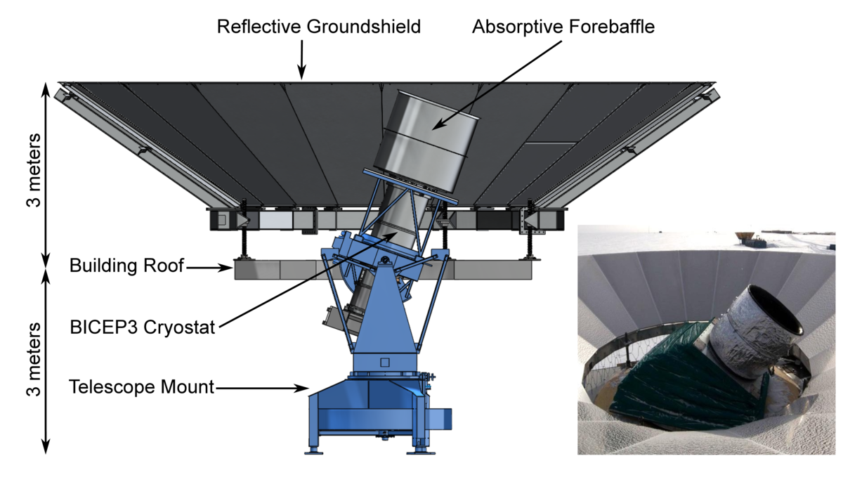
| BICEP3 telescope in the mount |
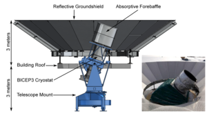 |
Figure 1: The BICEP3 telescope in the mount, looking out through the roof of the Dark Sector Laboratory (DSL) located \(\sim 800\)m from the geographic South Pole.
The insulating environmental shield shown in the bottom right photo is hidden in the CAD layout.
The three-axis mount previously used in BICEP1 and BICEP2 allows for motion in azimuth, elevation, and boresight rotation.
A co-moving absorptive forebaffle extends skyward beyond the cryostat receiver to intercept stray light outside the designed field-of-view.
Additionally, the telescope is surrounded by a stationary reflective ground shield which redirects off-axis rays to the cold sky.
| PDF / PNG |
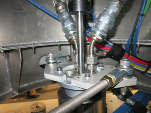
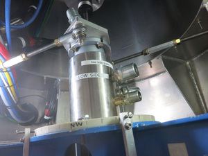
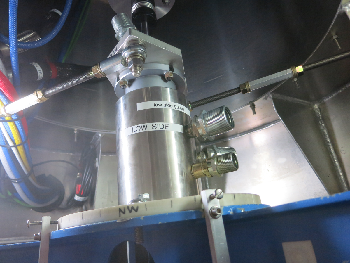
| Helium rotary joint system |
|
Figure 2: Photos of the 4-channel helium Rotary Joint system. Left: Two 30-degree bends rotate with the azimuth axis and go on to the receiver through the elevation and boresight axes. Right: Static section with the 4 connections for the high and low pressure helium and their respective guard channels. In both photos, two ball-end rod joints act as torque arms to transmit the azimuth rotation to the rotor of the HRJ.
| PDF1 / PNG1, PDF2 / PNG2 |
| Optical ray diagram |
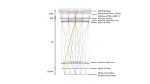 |
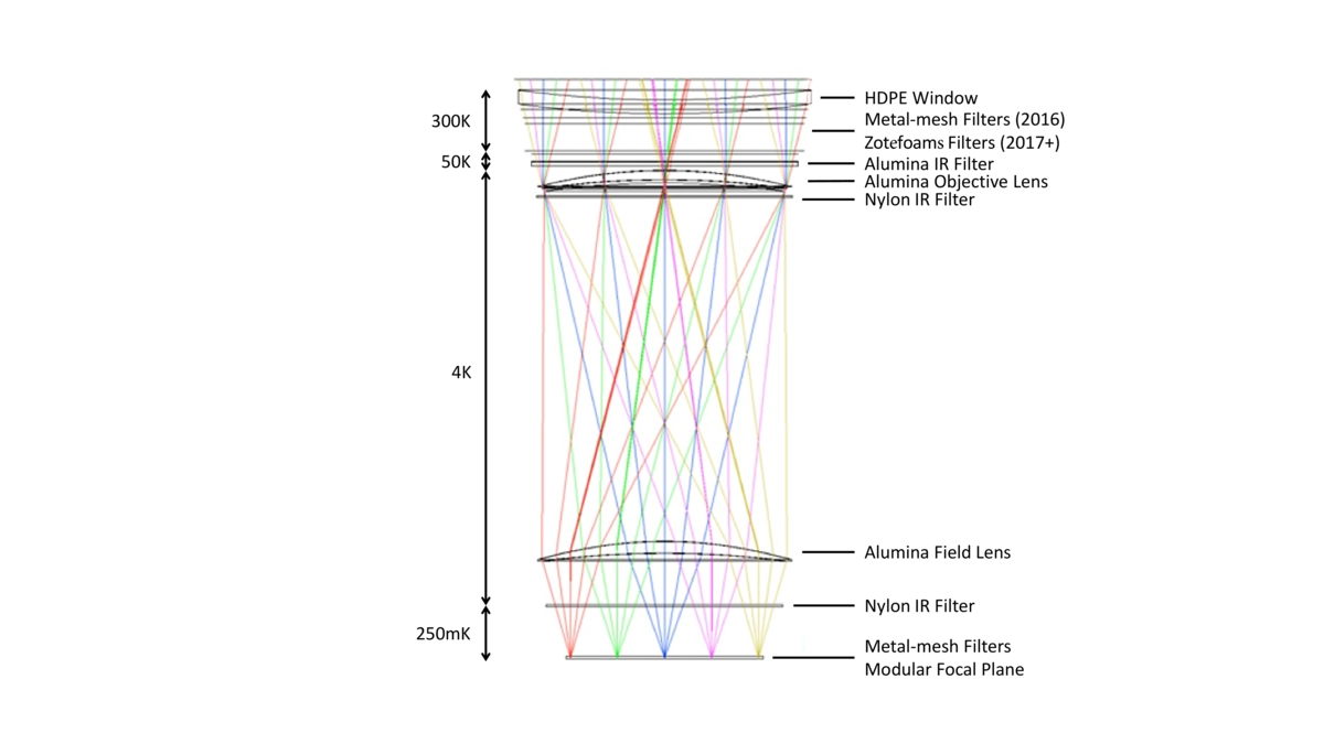
Figure 3: Ray diagram including the elements of the optical chain.
The 300K metal-mesh filters were replaced by a stack of 10 Zotefoam filters in 2017, which improved both the IR loading on the cryostat, and the in-band power incident on the detectors.
| PDF / PNG |
| Zotefoam filters |
 |
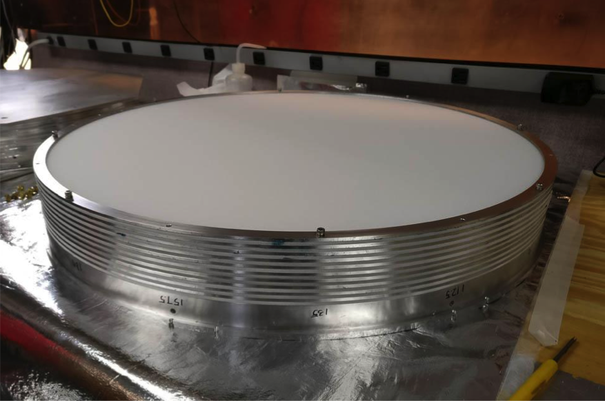
Figure 4: Stack of 10 layers room temperature IR filters installed in BICEP3, immediately behind the vacuum window.
This photo shows the current configuration, with each layer composed of 3.17mm thick HD-30 foam, glued onto a stack of aluminum frames with 3.17mm spacing.
The original design was a stack of metal-mesh filters, which was replaced in 2017.
| PDF / PNG |
| Alumina filter |
 |
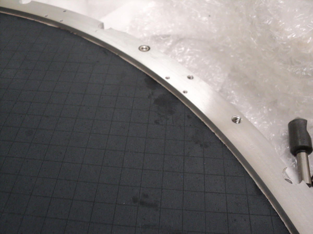
Figure 5: AR coated alumina filter in BICEP3.
The alumina filter is coated with a mix of Stycast 1090 and 2850FT.
The epoxy is machined to the correct thickness and laser diced to 1cm squares to mitigate differential thermal contraction between alumina and the epoxy.
| PDF / PNG |
| BICEP3 receiver |
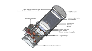 |
Figure 6: Cutaway view of the BICEP3 cryogenic receiver.
The thermal architecture is separated into a two-stage pulse tube cryocooler
(50K, 4K stages) and a three-stage helium sorption fridge
(2K, 350mK, 250mK stages).
All thermal stages are mechanically supported by sets of carbon fiber and G-10 fiberglass support.
The focal plane, with 20 detector modules and 2400 detectors, is located at the 250mK stage, surrounded by multiple layer of RF and magnetic shielding.
| PDF / PNG |
| BICEP3 sub-Kelvin stages |
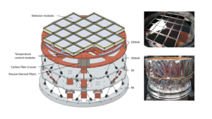 |
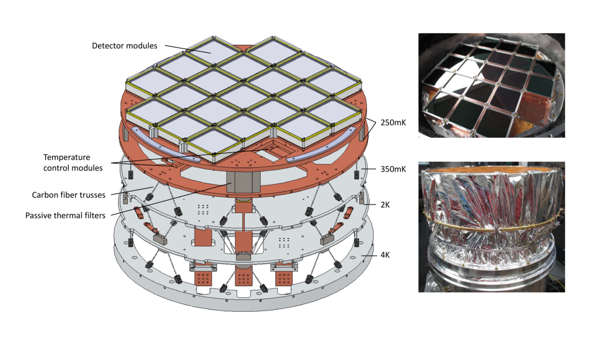
Figure 7: Left: Exploded view of the BICEP3 sub-Kelvin stages.
Each temperature stage is mechanically supported by sets of carbon fiber trusses.
Sets of stainless steel supports connect the two 250mK copper plates,
passively low-pass filtering thermal fluctuations,
and two active temperature control modules maintain thermal stability over observation cycles.
Right, top: The assembled focal plane with 20 detector modules
installed into the 250mK stage without metal-mesh edge filters.
The empty module slot in the lower right is absent due to the capacity of the readout electronics.
Right, bottom: A thin aluminized Mylar shroud extends from the top of the
focal plane assembly to the bottom of the 4K plate to close the 4K Faraday cage.
| PDF / PNG |
| Dark SQUIDs map |
 |
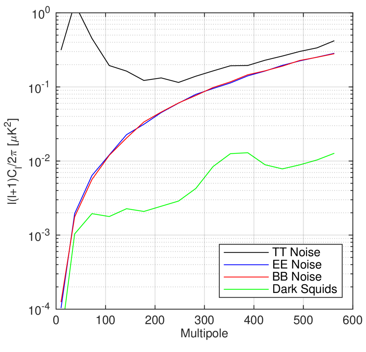
Figure 8: Temperature (black) and polarization (red and blue) noise of BICEP3.
The dark squids (green) is a readout channel that is disconnected from the detector, but sensitive to external magnetic field. This comparison demonstrates the magnetic pickup in science data is subdominant.
| PDF / PNG |
| Focal plane layout |
 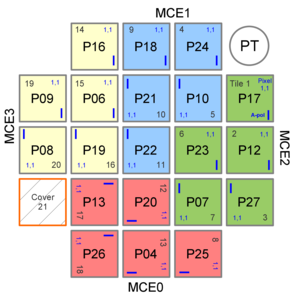 |
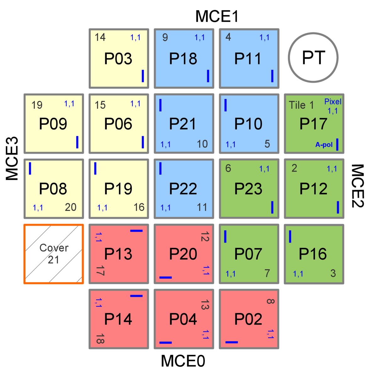
Figure 9: Left: BICEP3 focal plane layout in 2016.
Right: 4 modules were replaced prior to the 2017 season.
In each detector module, the serial number Pxx is labeled in the center.
The orientation of the module is indicated by the pixel (1,1) and the polarization A direction in blue, along with the tile number 1-20.
The background color of the module indicates the 4 readout MCE units.
The location of the pulse-tube cooler is shown by the PT marking in the upper right.
Slot 21, shown in an orange outline, does not contain a detector module, since the readout electronics were designed to support 20 modules.
It was covered with a thin copper sheet, which created extra reflection for Tile 1 as discussed in Sec. 8.10.
| PDF1 / PNG1, PDF2 / PNG2 |
| Exploded view of BICEP3 module |
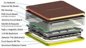 |
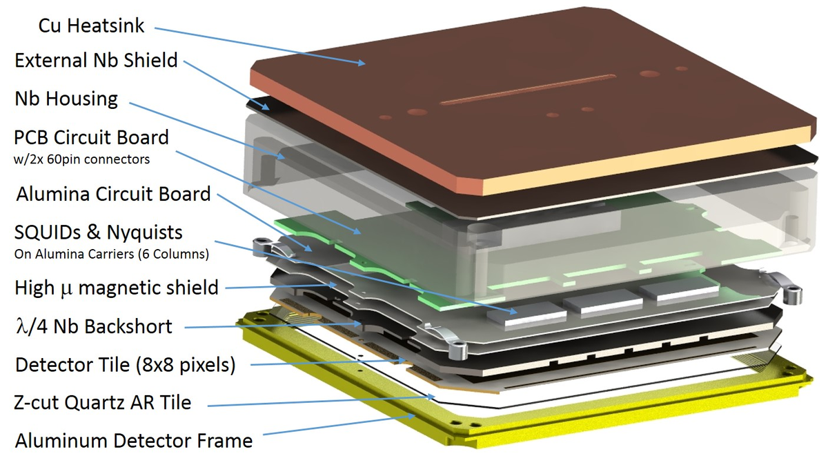
Figure 10: Exploded view of the BICEP3 detector module.
Sky-side is facing downward in this diagram.
The multiplexing SQUIDs and circuit boards are mounted directly behind the detector wafer, separated by a \(\lambda /4\) Nb backshort and A4K magnetic shield.
The backside is enclosed by a Nb cover and plate for magnetic shielding.
| PDF / PNG |
| Backside of BICEP3 module |
 |
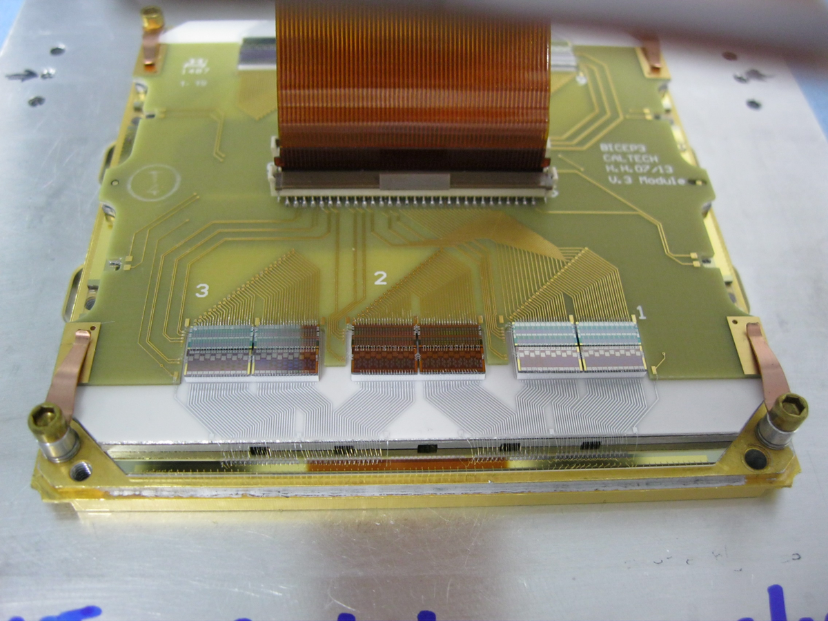
Figure 11: Backside of the detector module.
Aluminum wirebonds connect the detectors to SQUIDs chips via an alumina circuit board.
Two 60-pin Kapton/Cu flex-circuit ribbon cables connect to the ZIF connectors and travel out of the niobium casing through a thin slot to matching connectors on the focal plane board.
| PDF / PNG |
| COMSOL simulation of the module |
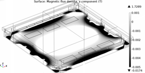 |
Figure 12: COMSOL Multiphysics simulation of the detector module, the scale is saturated to highlight the location of the SQUIDs (MUX).
Simulation shows the external magnetic field is reduced to \(\sim0.1\%\) at the SQUIDs.
| PDF / PNG |
| Simulation of corrugated frame |
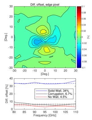 |
Figure 13: Top: Simulated peak normalized differential beam map for an edge pixel closest to the corrugation frame over 25% bandwidth at 95GHz.
Bottom: Peak-to-peak differential beam amplitude over design frequency band.
Solid lines are the simulated value, and dash lines are the average value over the 25% bandwidth.
Red lines show the case without metal frame, black lines show the current corrugated frame design, and blue lines show the pixel next to a solid metal wall.
This modeling is confirmed by our measurements shown in the middle panel of Fig. 23.
| PDF / PNG |
| MUX11 circuit diagram |
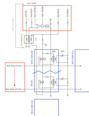 |
Figure 14: MUX11 SQUID readout and feedback schematic modified from Fig. C.1 in Grayson (2017), explicitly showing two RS of one MUX column.
Red outlines denote MCE-sourced signals at 300K, green the SSA modules at 4K, and blue the MUX chips at 250mK.
This diagram does not show the Nyquist chip outline or the Nyquist inductor.
A single bias line is used to bias both the SQ1 and the flux switches (FS).
| PDF / PNG |
| Spectral response |
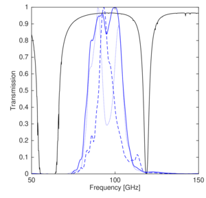 |
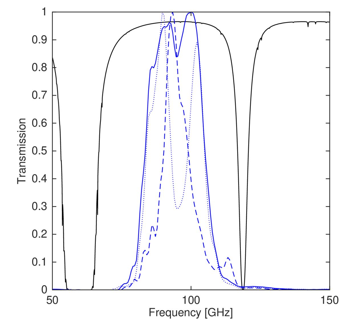
Figure 15: The peak-normalized, average spectral response of BICEP3 detectors
(solid blue) shown against the atmospheric transmission at the South Pole (black).
Also plotted are two extreme example cases of the type of bandpass variation caused
by delamination of the low-pass edge filters in 2016:
a spike-like spectrum (dashed blue, \(e=-0.51\)) and
a dip-like spectrum (dotted blue, \(e=0.20\)).
All low-pass edge filters were replaced for the 2017 season,
and subsequent measurements are similar to the average spectrum for all detectors.
| PDF / PNG |
| Spectral estimator |
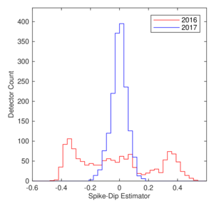 |
Figure 16: The spectral (spike-dip) estimator e with the 2016 and 2017 focal planes, calculated with Eq. 4.
The peaks in \(e=\pm\sim0.4\) indicate that many detectors in the 2016 focal plane exhibited spike and dip-like features.
| PDF / PNG |
| Optical efficiency |
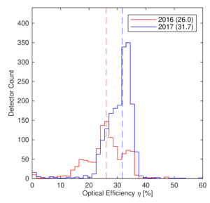 |
Figure 17: Optical efficiencies of BICEP3 detectors.
The median efficiency increased from 26% in 2016 (red) to
32% in 2017 (blue).
Because the optical efficiency measurement is performed with the detectors biased on the aluminum transition, the detector yield shown here is lower than the yield for CMB observations, when the detectors are biased on the titanium transition.
| PDF / PNG |
| Time constant |
 |
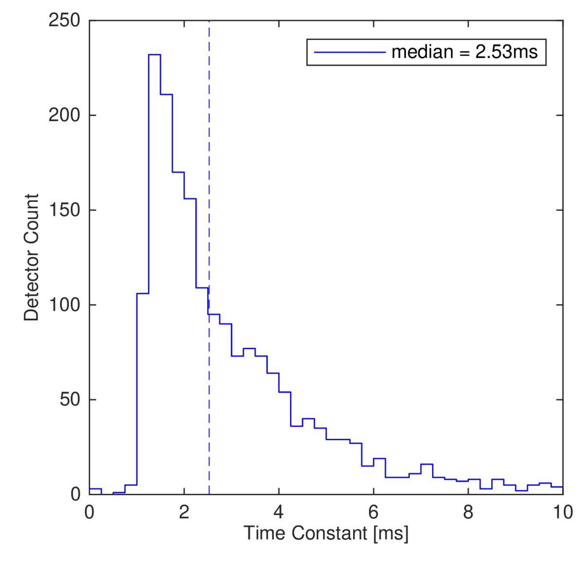
Figure 18: Detector time constants in 2021, measured at the nominal TES bias voltage used for CMB observations.
| PDF / PNG |
| NET vs bias |
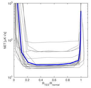 |
Figure 19: Noise equivalent temperature (NET) in units of CMB temperature as a function of detector resistance.
The gray lines are the NET for each detector in one sample readout column, and the blue line is the average response for that column.
The optimal bias point for the readout column is determined when average NET is at its minimum.
The "noise stares" were taken under conditions of low atmospheric loading with an assumed sky temperature.
Variation in sky temperature will affect the absolute NET values shown in this figure, but do not impact the selection of optimal bias point.
| PDF / PNG |
| Crosstalk |
 |
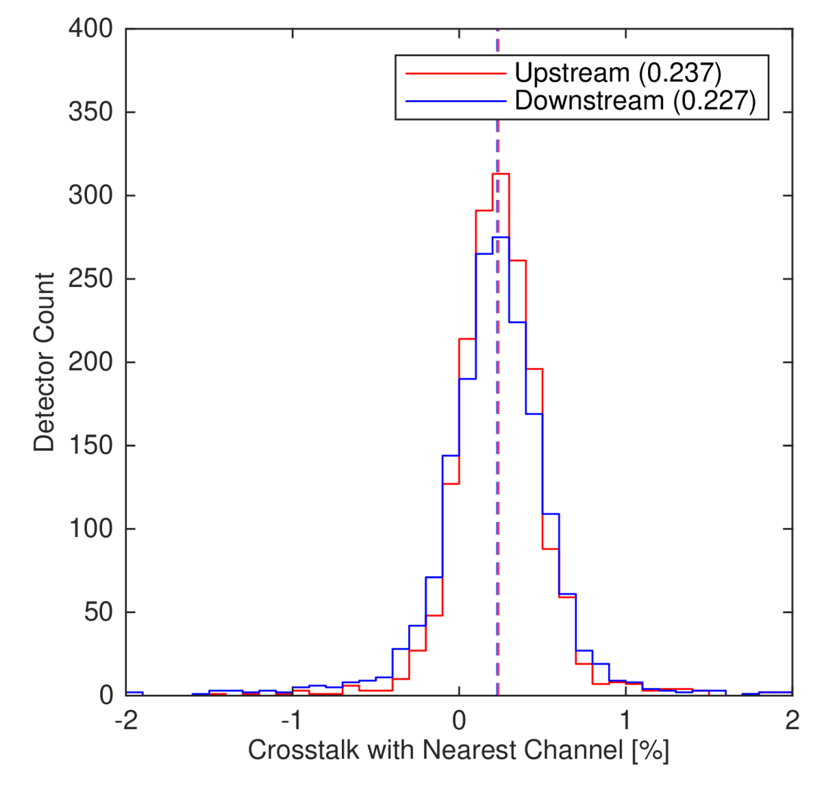
Figure 20: Measured nearest-neighbor crosstalk in each detector using a cosmic ray analysis with median value shown in parentheses.
The red histogram shows upstream crosstalk (response seen in the detector visited before the target detector in the time domain) and the blue histogram shows downstream crosstalk (response seen in the detector sampled after the target detector).
| PDF / PNG |
| Detector noise model |
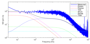 |
Figure 21: Measured and modeled noise for a nominal single undifferenced detector in BICEP3.
We plot noise equivalent current (NEI) in the SQUID and readout electronics.
The noise in Eq.9 and 10 have NEP=NEI/S, where the responsivity \(S=dI/dP=1/V*\mathscr{L}/(\mathscr{L}+1)*1/(1+j\omega\tau)\), \(\mathscr{L} \geq10\) and the effective time constant \(\tau\) is measured to be \(\tau\sim 2\)ms (Fig. 18). The 1/f knee at 8Hz in the measured spectra is from atmospheric fluctuations, which is suppressed by an order of magnitude down to 0.1Hz after pair-difference polarization pairs (see Fig. 33).
The 1/f knee at 8Hz in the measured spectra from atmospheric fluctuations, which are suppressed by an order of magnitude to 0.1Hz in pair-difference polarization pairs.
| PDF / PNG |
| Near-field beam centers |
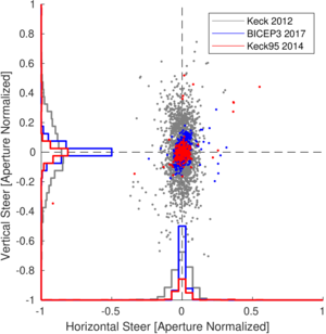 |
Figure 22: Near-field beam centers of BICEP3 detectors for the 2017 observing season (blue) compared to those of all Keck 150GHz focal planes in 2012 (gray) and all Keck 95GHz focal planes in 2014 (red).
The new "etch-back" procedure in detector fabrication was implemented after 2012.
| PDF / PNG |
| Near-field beam maps |
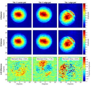 |
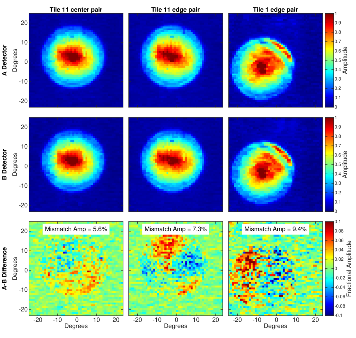
Figure 23: Amplitude-normalized near-field beam maps for detector pairs individually (top and middle rows) and their difference beams (third row) for a pair at the center of both the focal plane and its respective tile (left column); a pair near the center of the focal plane but at the edge of its tile (middle column); and a pair that is both at the edge of its tile and the whole focal plane.
The pair centered both in the tile and focal plane demonstrates the minimum typical A/B mismatch that can be expected by detectors under ideal conditions.
The pairs central on the FPU but at the edge of the tile confirms both the level and shape of the simulations in Fig.13 where differential pointing is slightly exacerbated by the proximity of a detector pair to the corrugation frame.
The pair at the edge of both the FPU and its tile demonstrates how a small subset of beams near the edge are steered into the aperture stop, which we attribute to beam truncation at the camera lens.
| PDF / PNG |
| Far-field beam map |
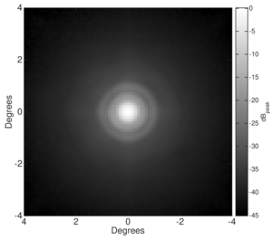 |
Figure 24: The BICEP3 average beam, made by coadding composite beam maps
from all optically-active detectors.
| PDF / PNG |
| RPS |
 |
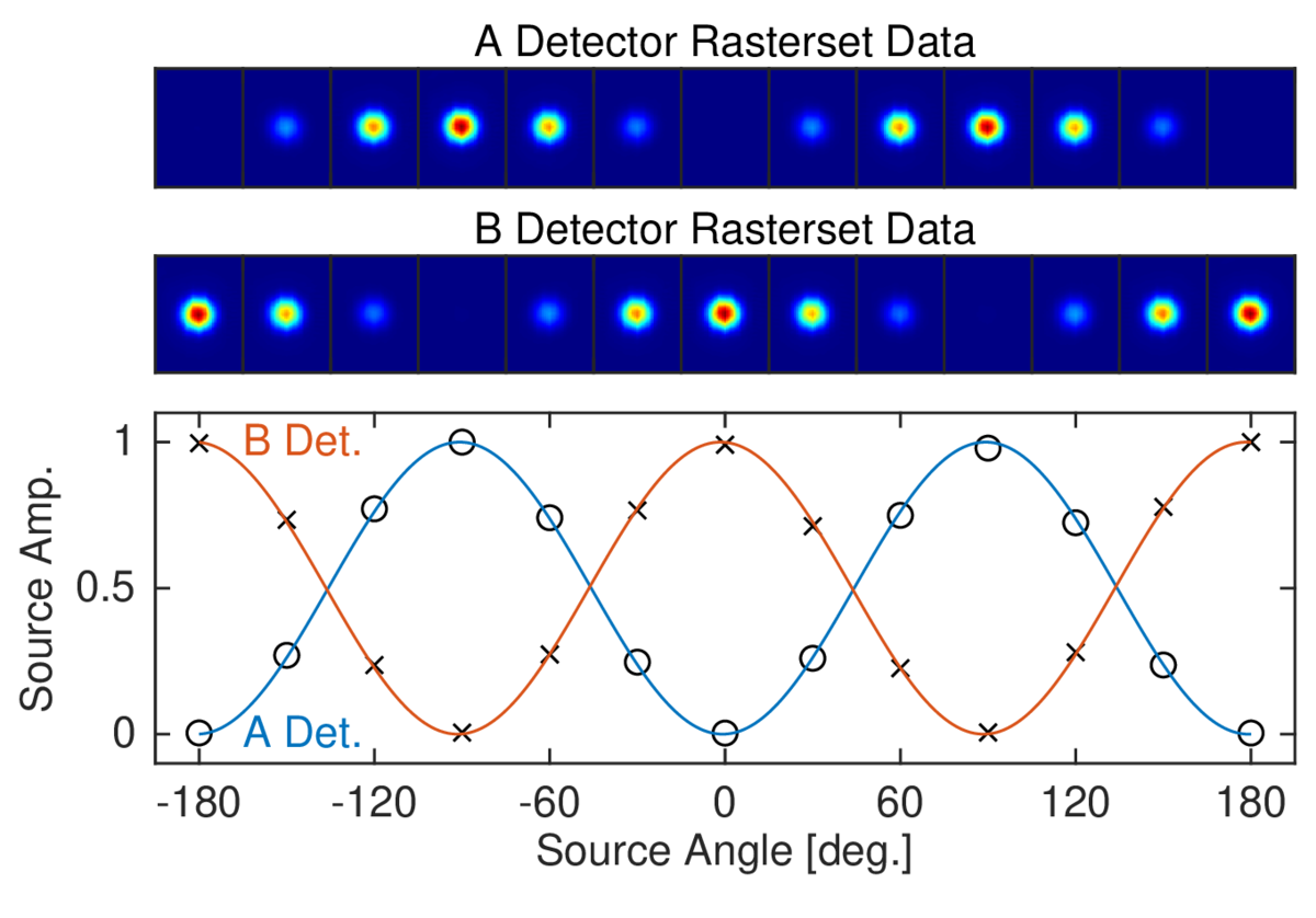
Figure 25: Beam maps of individual RPS rasters for an A/B-polarization detector
(top/middle) and the corresponding normalized modulation curve
(bottom), where the blue and orange lines are the best-fits to the
A- and B-polarization detectors, respectively.
| PDF / PNG |
| Far-sidelope map |
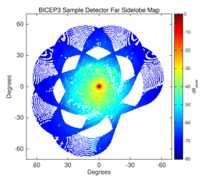 |
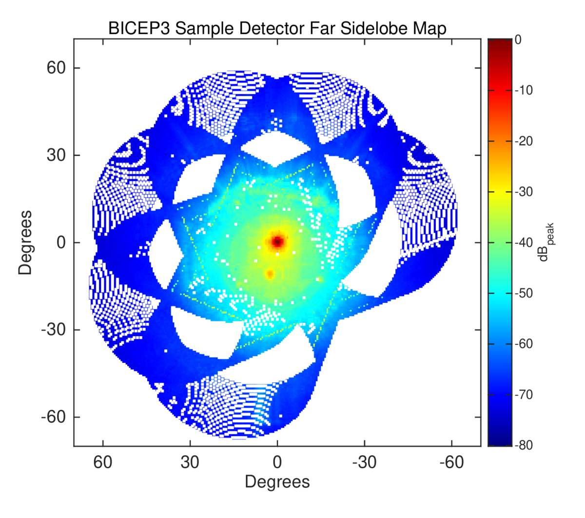
Figure 26: Sample far-sidelobe map of a BICEP3 detector, made by stitching together measurements from three power settings and coadding maps made at both source polarization orientations.
The forebaffle was on for this measurement, representing the true beam response on sky as during CMB observations.
The main beam and extent of the BICEP3 aperture are clearly seen.
The feature just below the main beam in the map is the "ghost" beam described in the text.
| PDF / PNG |
| Ghost beam ratio |
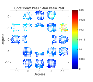 |
Figure 27: Per-pair values of the ratio of ghost beam peak power to the main beam peak power.
Each point is the average between both detectors in a pair.
For detectors near the center of the focal plane, ghost beams cannot be confidently separated from the main beam and are therefore omitted from this plot.
Tile 1 (top-right corner) has higher-amplitude ghost beams due to the increased reflection from the blanked port on the opposite side of the focal plane.
| PDF / PNG |
| Observation field |
 |
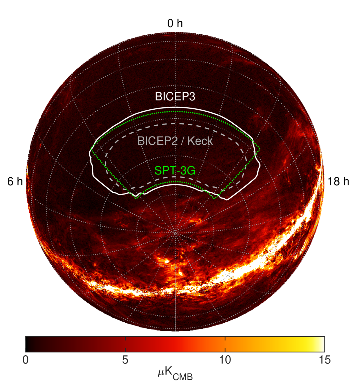
Figure 28: The BICEP3 CMB observing field (solid white) on the southern
celestial sphere, together with the smaller BICEP2/Keck field (dashed white) and the
SPT-3G \(1500~\text{deg}^{2}\) survey (dotted green).
The background image shows the polarized intensity \(P = \sqrt{Q^2 + U^2}\)
of the Planck component-separated (SMICA) dust map,
rescaled in amplitude from \(353\,\mathrm{GHz}\) to \(95\,\mathrm{GHz}\)
assuming a graybody spectrum with temperature
\(T_\mathrm{d} = 19.6\,\mathrm{K}\) and spectral index \(\beta_\mathrm{d} = 1.5\).
| PDF / PNG |
| Observation schedule |
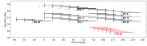 |
Figure 29: Observing pattern of a typical three-day schedule in ground-based coordinates.
The first scanset of phase F is shown in bold.
Horizontal lines indicate the field scans and the vertical lines indicate the bracketing elevation nods.
The telescope scans at a fixed elevation during each scanset.
For the CMB field scans, we observe two scansets before changing elevation.
Phase D is on the galactic plane.
| PDF / PNG |
| Observation efficiency |
  |
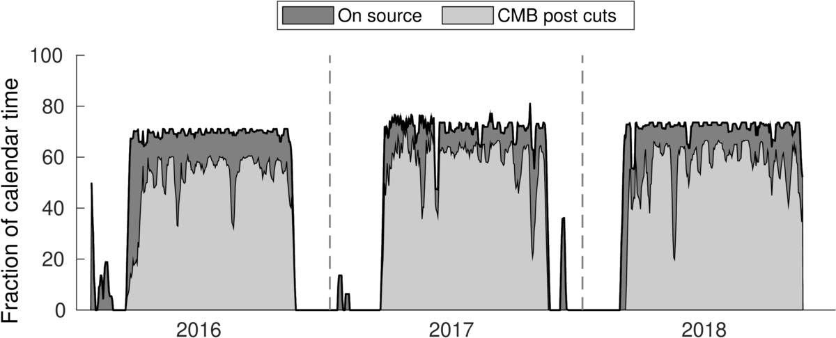
Figure 30: Integration of the BICEP3 data set from 2016 to 2018, plotting (top) fraction of time per day spent in CMB scans, excluding regular calibrations and refrigerator cycling.
During austral summers (November to February), the observing schedules were been interspersed with calibration measurements.
During the austral winter, on-source efficiency is about 70%.
The lower curve includes data quality cuts, but excluding non-functioning channels.
The rms map-based sensitivity (bottom) improves over time and reaches \(2.8\mu\text{K}_{\text{arcmin}}\) at the end of 2018.
| PDF1 / PNG1, PDF2 / PNG2 |
| Distributions of jackknife \(\chi\) and \(\chi^2\) PTE values |
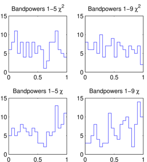 |
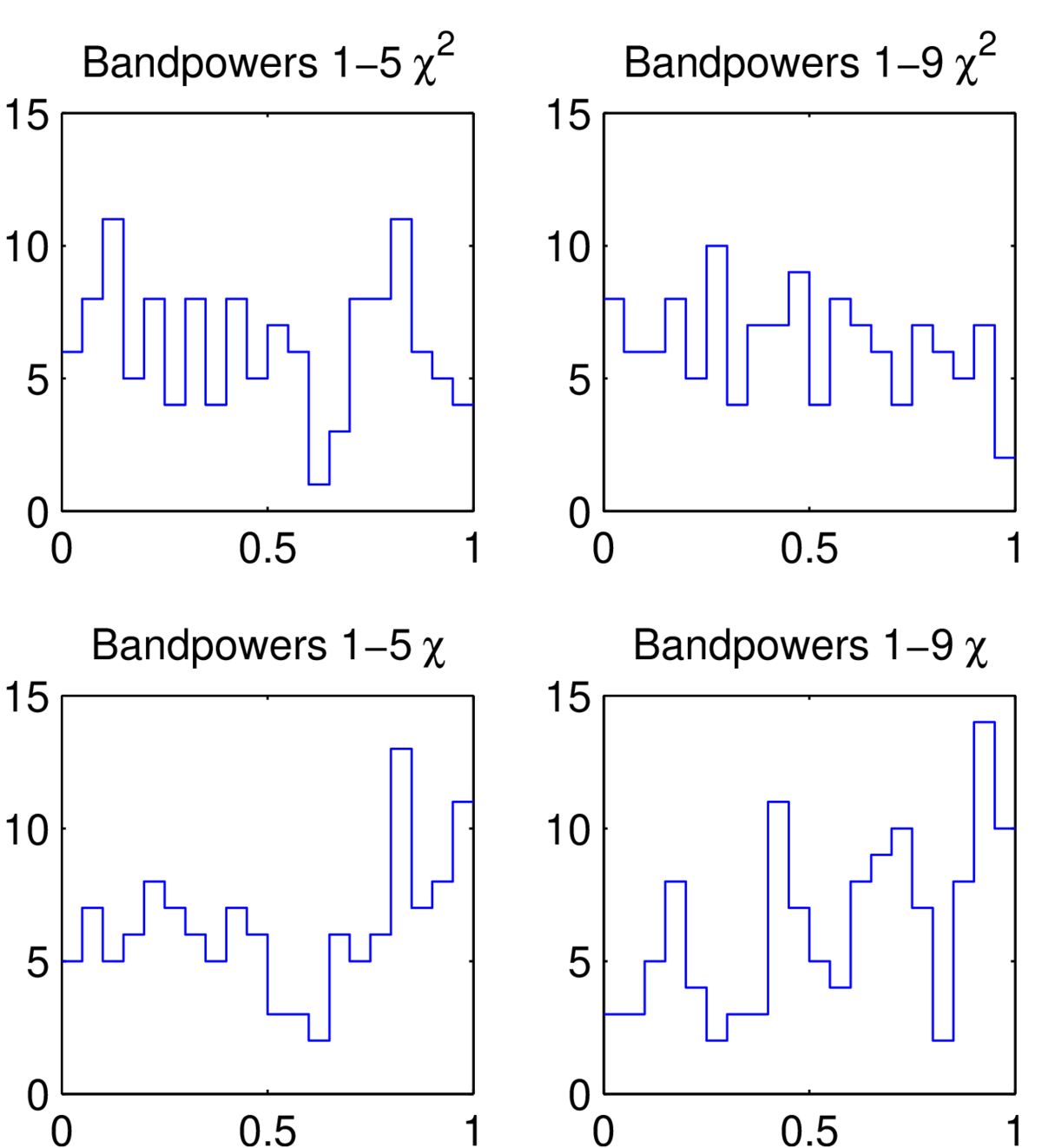
Figure 31: Distributions of the jackknife \(\chi\) and \(\chi^2\) PTE values for BICEP3 2016 to 2018 95GHz data.
They are consistent with a uniform distribution, indicating there is no evidence for systematics at the level of statistical sensitivity.
| PDF / PNG |
| 2016 spectral jackknife |
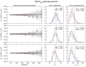 |
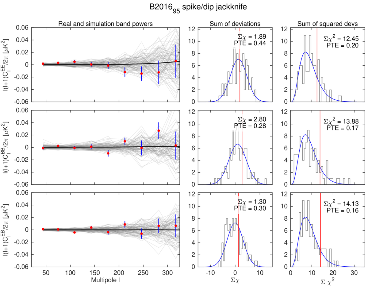
Figure 32: Left: Bandpowers for the BICEP3 2016 spike-dip jackknife EE, BB, and EB spectra.
The welter of light gray lines are the bandpowers of the ensemble of 99 lensed-\(\Lambda\)CDM+dust+noise simulations, with the mean of these simulations given by the thick black line.
The real map bandpowers are given by the red circles, where the error bars are for the standard deviation of the simulations.
Right: Histograms of the \(\chi\) and \(\chi^2\) statistics for each simulation, with the expected Gaussian and \(\chi^2\) distribution over-plotted in blue.
The real data value is marked by the vertical red line, with the value and corresponding probability to exceed (PTE) annotated.
| PDF / PNG |
| Per detector noise spectra |
 |
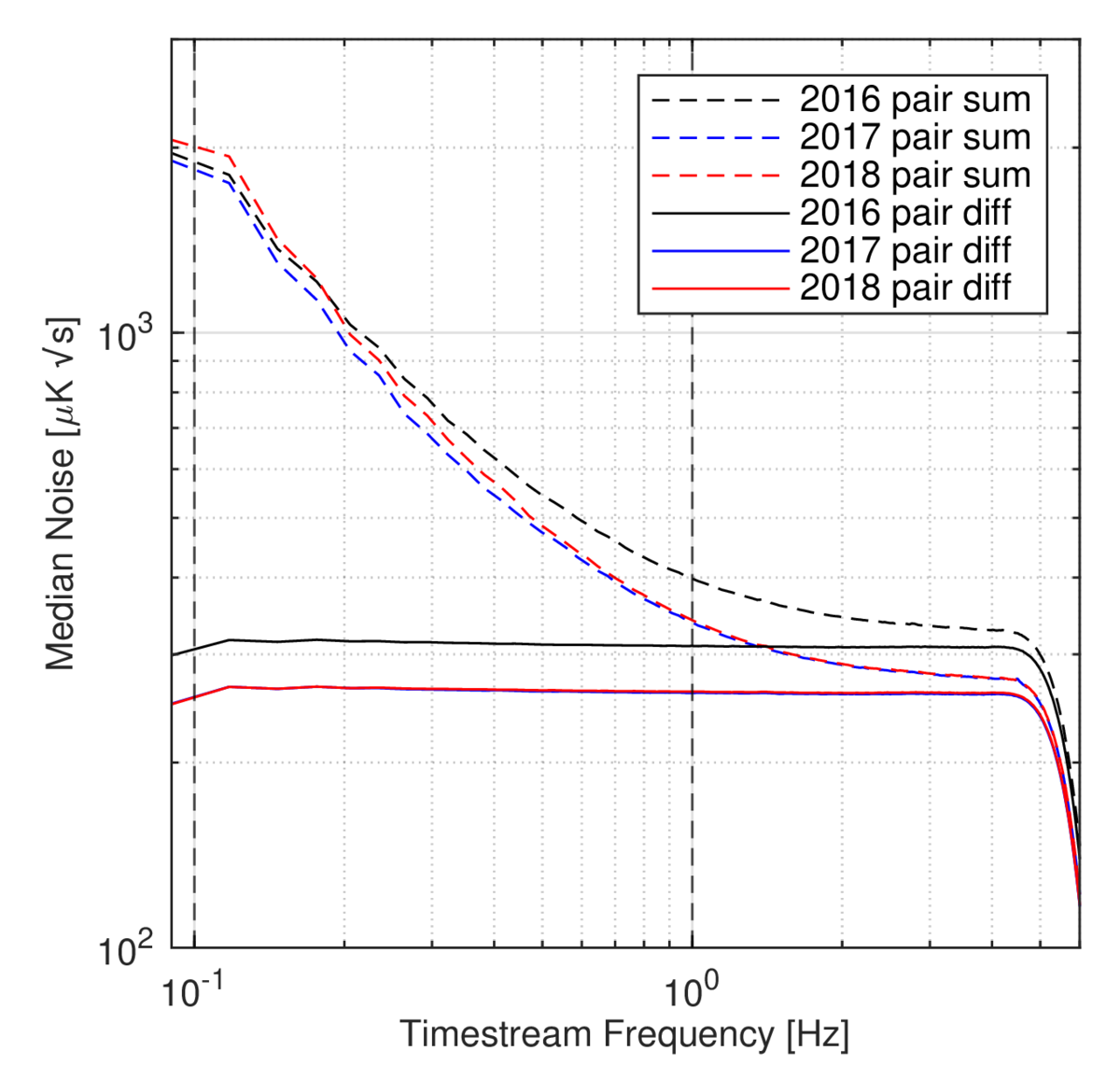
Figure 33: Median pair-sum and pair-diff noise spectra, evaluated from minimally-processed timestreams from the BICEP3 2016-2018 seasons.
The median per-detector NET is the average between the science band from 0.1-1Hz.
| PDF / PNG |
| Histogram of per-detector, per-scanset NET |
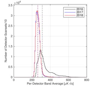 |
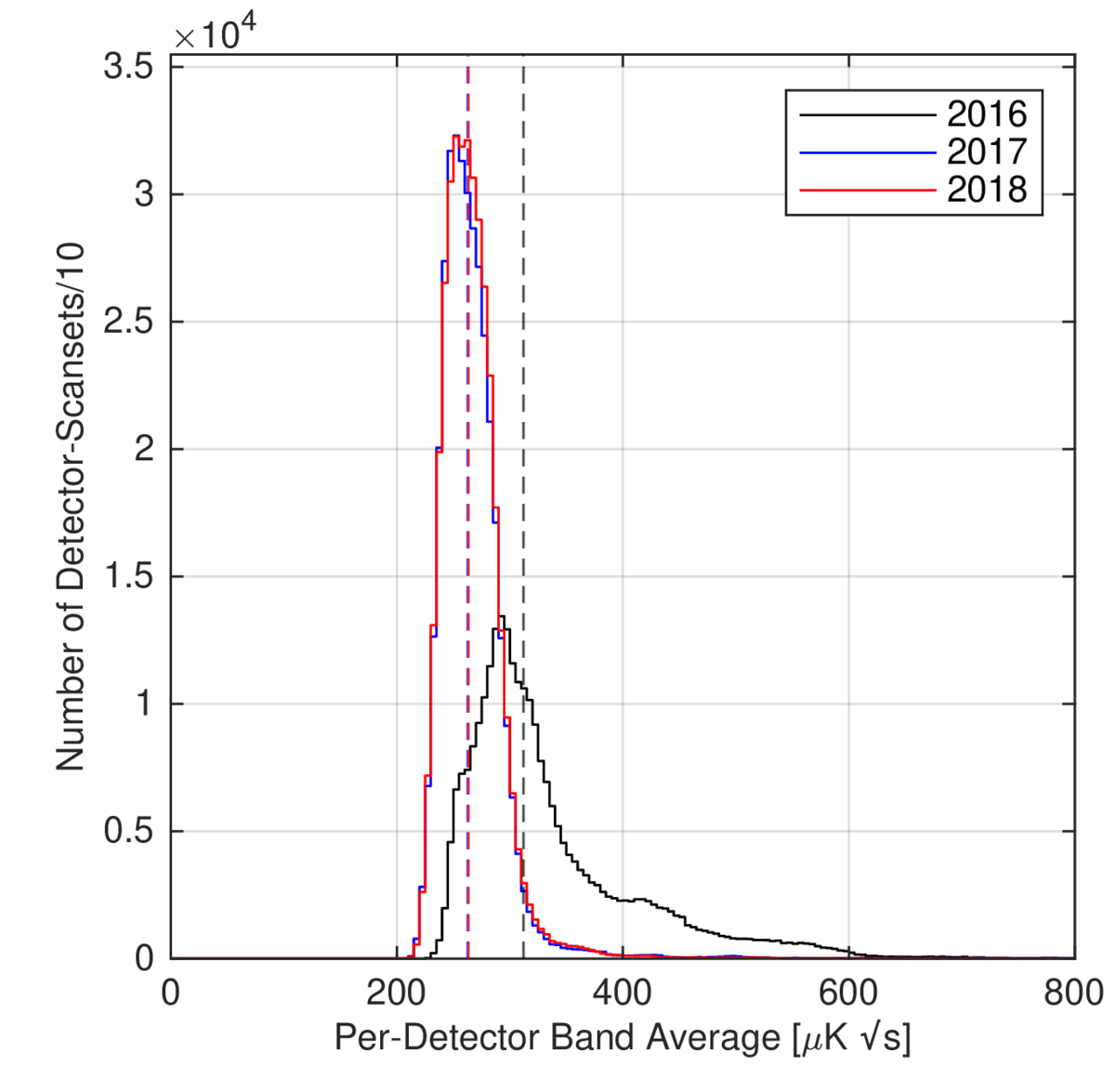
Figure 34: Histogram of per-detector, per-scanset noise for every 10th scanset from 2016 to 2018, after applying a 3rd-order polynomial filter and averaging across the 0.1-1Hz science band.
Median values of \(312\mu\text{K}_{\text{CMB}}\sqrt{\text{s}}\) and \(263\mu\text{K}_{\text{CMB}}\sqrt{\text{s}}\) are marked by vertical dashed lines for the 2016 and 2017/18 data, respectively.
The reduced internal receiver loading after switching from the metal-mesh infrared filters to the Zotefoam filters, as well as swapping four detector modules, leads to the improved noise performance shown here.
| PDF / PNG |
| 3 years T/Q/U maps |
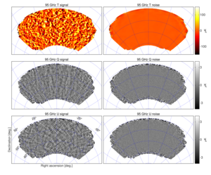 |
Figure 35: T, Q, U map and its jackknife using the 3-years dataset from BICEP3.
E-mode polarization is measured to high S/N, evidenced by visually seeing the \(+\) and \(\times\) patterns in the Q and U maps.
| PDF / PNG |