| Setup for far-field beam mapping |
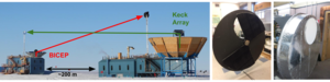 |
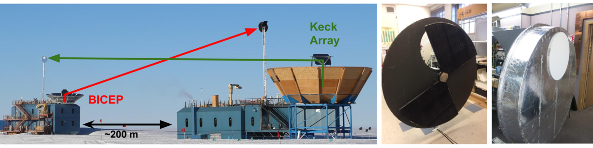
Figure 1: Several weeks of each South Pole deployment season are spent generating far-field beam maps using the pictured setup. Left: Keck Array and BICEP3 taking far-field beam maps simultaneously at South Pole. Both choppers and far-field flat mirrors are visible. Middle: Carbon fiber chopper blade coated in Eccosorb HR-10, mounted in the lab; during operation it spins at 14 Hz. Right: Carbon fiber enclosure holding the blade; the 60 cm aperture (white) is sealed with Zotefoam HD30. When the blade does not fill the aperture, the beam is redirected to the zenith with a 45° mirror.
|
PDF / PNG |
| Coordinate system schematic |
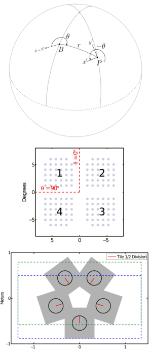 |
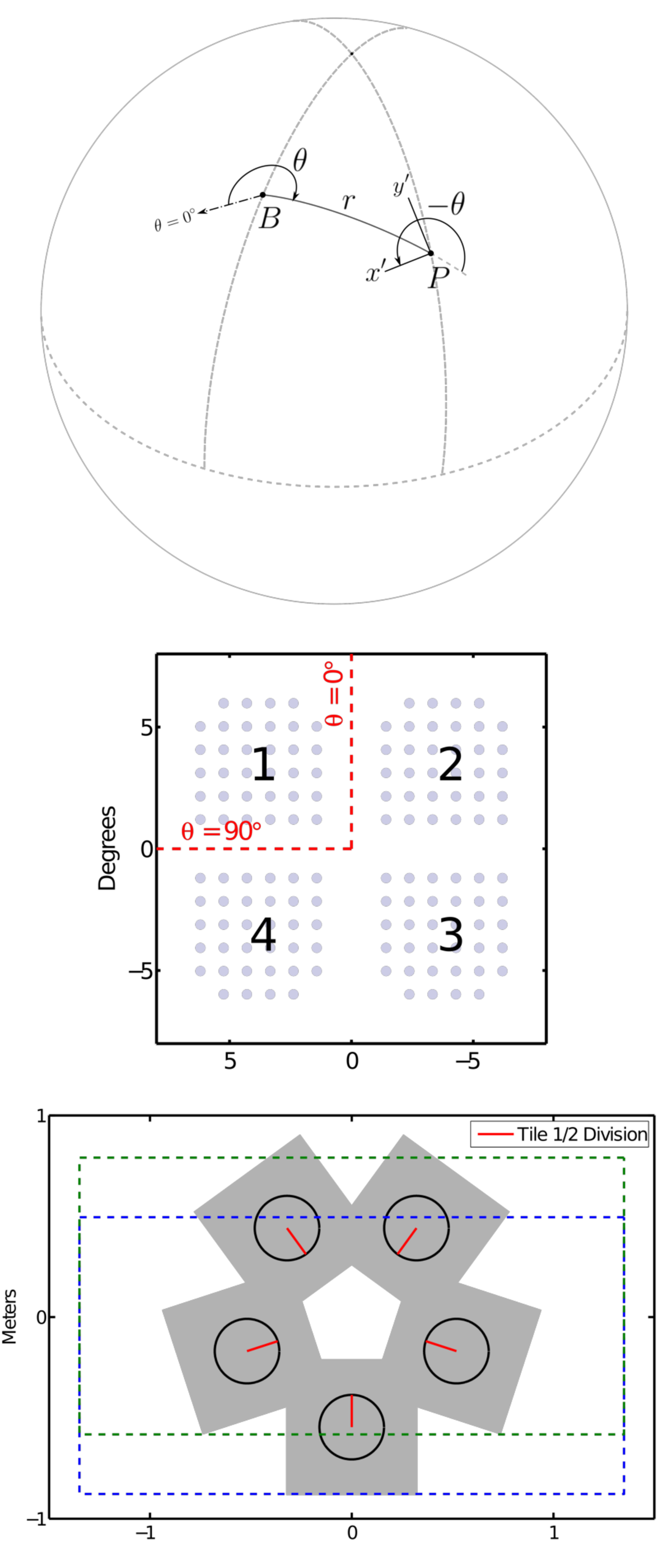
Figure 2: Top: the (x′, y′) coordinate system is centered locally for each pixel P at a location (r, θ) from the boresight B, and is referenced to the θ = 0° ray. Middle: the θ = 0° ray is referenced to the orientation of the detector tiles, here depicted looking directly down onto the focal plane. Bottom: schematic of the five Keck receiver apertures in the mount, clocked at 72° with respect to each other. Each receiver's Tile 1/2 dividing line (corresponding to the θ = 0° ray) is indicated. Two footprints of the far-field flat mirror (hoisted 3.7 m above the apertures) are depicted as dashed boxes. The rough extent to which the beams have diverged by the time they intercept the mirror is depicted in gray. Multiple mirror positions are necessary to reflect beams from all receivers at many boresight angles.
|
PDF / PNG |
| Keck Array differential pointing and ellipticity |
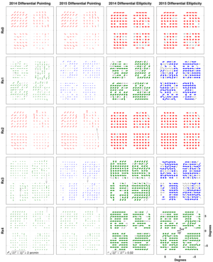 |
Figure 3: Differential pointing and ellipticity for Keck Array receivers in the 2014 and 2015 seasons. Parameters are plotted in focal plane coordinates as projected on the sky. A/B detectors are polarized along the y′/x′ axes respectively, indicated in the bottom right panel. Detectors at 95 GHz are in red, 150 GHz in green, and 220 GHz in blue; those in gray are not used in analysis. Parameters are consistent across years when the receiver did not change—Rx0, Rx2, and Rx4 stayed the same in 2014 and 2015. Left columns: Differential pointing rendered as an arrow pointing from the A detector location to the B detector location. The arrow length indicates the degree of mismatch, multiplied by 20. Right columns: Differential ellipticity rendered as ellipses; major axes are proportional to √p2 + c2, a measure of the magnitude of the differential ellipticity (minor axes are fixed). The magnitude has been multiplied by 75 for visibility. BK-IV presents analogous plots for BICEP2 and Keck Array in previous seasons.
|
PDF / PNG |
| Composite beam maps at 95, 150, and 220 GHz |
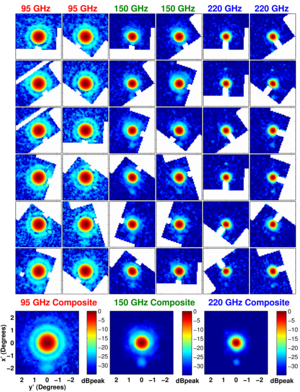 |
Figure 4: Large panels: example composite beam maps for individual 95 GHz (left), 150 GHz (middle), and 220 GHz (right) detectors. Small panels: the component maps that contribute to the composite, taken at multiple boresight angles—the ground, mast, and SPT have been masked out. The x′, y′ coordinate system is detector-fixed. The circular feature at the ∼−23 dB level, which in all cases here appears below the main beam, is due to crosstalk in the readout system and has been extensively characterized (BICEP2 Collaboration II 2014; BICEP2 Collaboration III 2015). The maps are in dB relative to peak amplitude and share the same color scale; because beams of different widths have different peak amplitudes, the noise in the lower-frequency beams appears inflated.
|
PDF / PNG |
| Beam profiles at 95, 150, and 220 GHz |
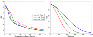 |
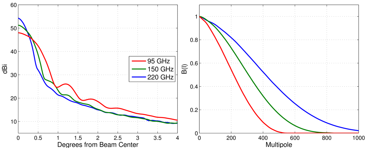
Figure 5: Left: azimuthally averaged beam profiles for Keck Array at 95, 150, and 220 GHz, coadded over all operational channels in 2015. The maps are normalized relative to an isotropic radiator under the assumption that all beam power is contained within the r < 4° maps. Right: The B(ℓ) window functions, equivalent to Fourier transforms of the beam profiles. The effect of the finite source size has been removed. BK-IV presents analogous plots for BICEP2 and Keck Array in previous seasons.
|
PDF / PNG |
| Differential beam maps at 95, 150, and 220 GHz |
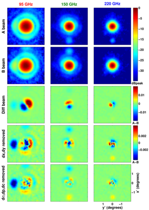 |
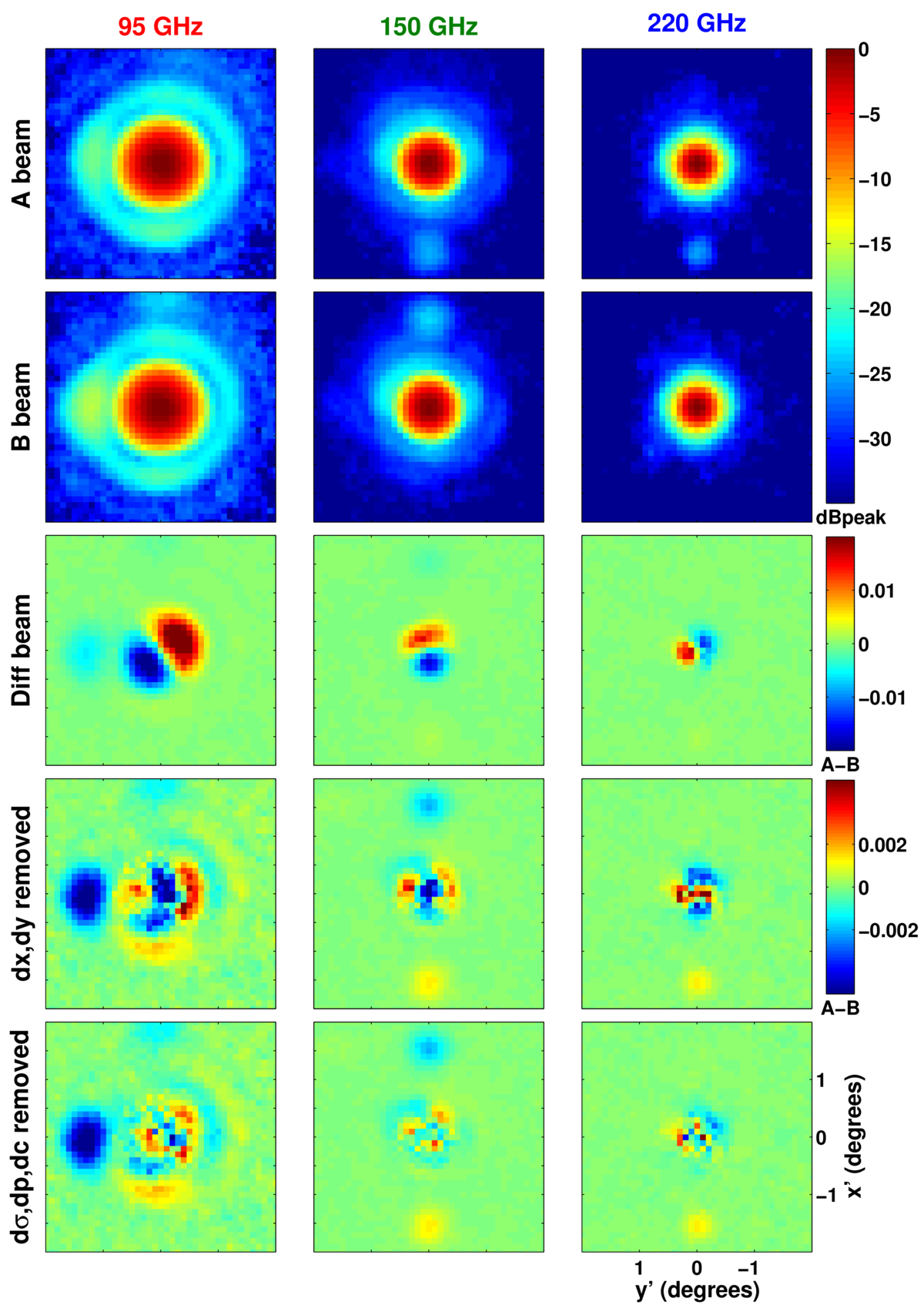
Figure 6: Example differential beam maps at 95 GHz (left), 150 GHz (middle), and 220 GHz (right). In each column, the top two panels show composite maps of A and B detectors in a pair; the color scale is in decibals relative to the peak amplitude. The third panel shows the difference between A and B, dominated by differential pointing. The color scale is linear relative to the pair sum peak amplitude (±2%). The fourth panel shows the residual after differential pointing is deprojected; note the color scale has changed (±0.5%). The last panel has the same color scale as the fourth and shows the undeprojected residual after differential pointing, beamwidth, and ellipticity have been removed; this contributes to the T→P leakage discussed in Section 5.2. The large feature in the 95 GHz map is discussed in more detail in the text.
|
PDF / PNG |
| Maps of T→P leakage |
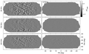 |
Figure 7: Apodized Q maps of T→P leakage predicted by the beam map simulations (left column) and a beam map noise realization (right column). The visible signal is due to higher-order undeprojected residuals in the measured differential beam maps and potentially systematics in the beam measurement. The leakage at 95 GHz is mostly E mode in character and is due to the anomalous feature in the 95 GHz tile edge pixels, shown in Figure 6. The band of lower leakage at the center of the 150 GHz map is due to the complex cancellation of the 17 receiver-years that compose the map.
|
PDF / PNG |
| BB power spectra from beam map sims |
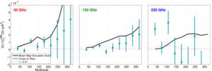 |
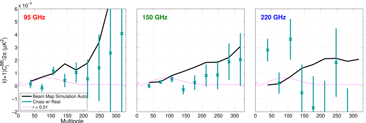
Figure 8: BB power spectra from beam map simulations, corresponding to the maps shown in Figure 7. The black lines are the per-frequency auto spectra, which have been noise-debiased using the beam map jackknife maps. They should be considered upper limits on T→P leakage. The teal crosses show the cross spectra of the beam map simulations with the BK15 maps. The error bars are derived from the cross spectra of the fixed beam map simulation with 499 CMB lensing + dust + instrumental/atmospheric noise simulations. Noise and systematics in the beam map measurement are not included in this error estimate.
|
PDF / PNG |
| Shifts in maximum-likelihood r for various T→P leakage and recovery scenarios |
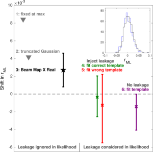 |
Figure 8: Shifts in maximum-likelihood r with respect to the baseline analysis for a set of 499 simulations, which have had varying levels of T→P leakage injected and with various recovery scenarios. The numbers refer to scenarios listed in Section 6.2. For scenarios 3–6, the 16th, 50th, and 84th percentiles are plotted. The inset panel shows histograms of rML for the baseline analysis (blue) and Scenario 3 (black) to emphasize that the potential bias due to T→P leakage is much smaller than the BK15 statistical error, σ(r) = 0.020.
|
PDF / PNG |