| Detector orientation matrix |
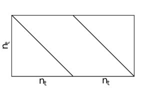 |
Figure 1: Detector orientation matrix, [α- β-]. The matrix is only filled on the diagonals of the two sub-blocks, α and β.
|
PDF / PNG |
| Timestream forming matrix |
 |
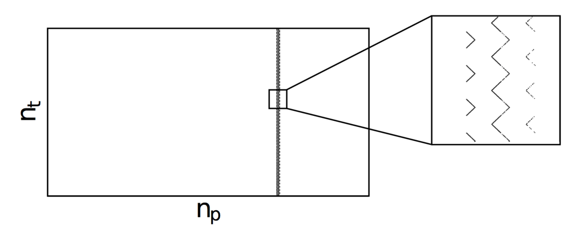
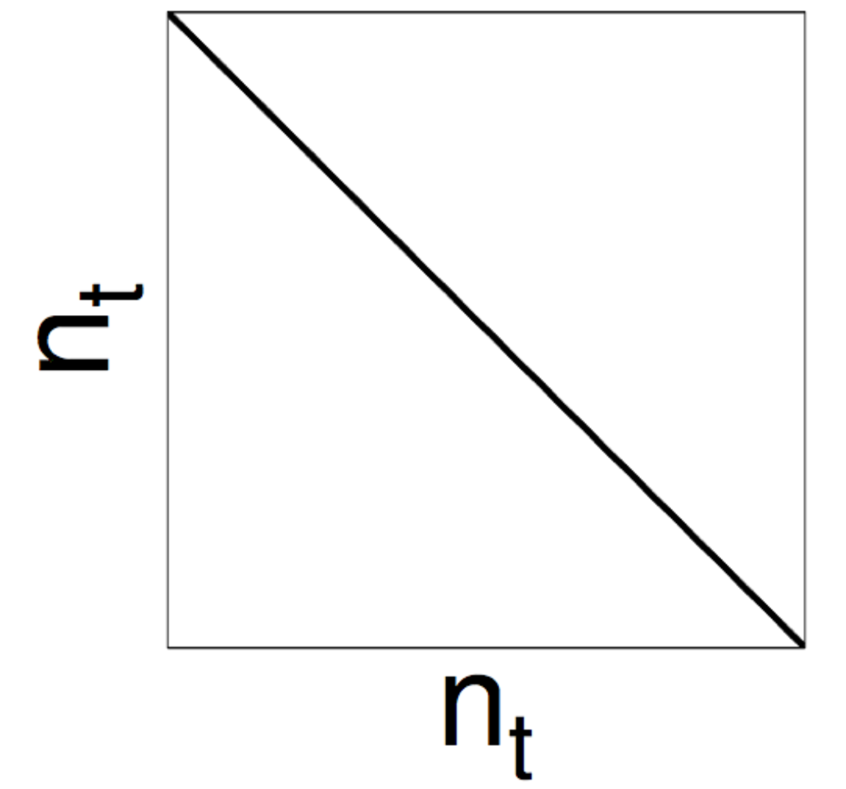
Figure 2: Timestream forming matrix, A: filled elements of the matrix that takes HEALPix maps to timestreams. This matrix contains the pointing of a single detector pair over one scanset within a Nside=512 HEALPix map. The pattern of the filled elements is determined by the particular HEALPix pixel indexing scheme. There are nt filled entries, consisting of a 1 for each timestream sample. Note that although the above image appears to have multiple pointing locations for a single timestream sample, nt, this is merely a result of the limited resolution in the image. The timestream forming matrix contains only one HEALPix pixel location for each time sample.
|
PDF / PNG |
| Polynomial filtering matrix |
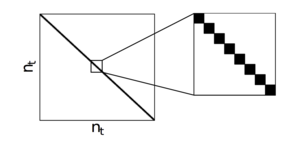 |
Figure 3: Polynomial filtering matrix, F, showing the filled elements of the matrix. The matrix is very sparse and is block diagonal with blocks the size of a halfscan (≈ 404 samples).
|
PDF / PNG |
| Scan-synchronous signal removal matrix |
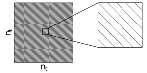 |
Figure 4: Scan-synchronous signal removal matrix, G, showing the filled elements. The scan-synchronous signal matrix is sparse Toeplitz, with off diagonal components that subtract the average scan-synchronous signal for one of the two scan directions in a scanset.
|
PDF / PNG |
| Weighting matrix |
 |
Figure 5: Weighting matrices w±, showing the filled elements. The weighting matrices are zero except on the diagonal, where they contain the weights based on the inverse variance of the timestream.
|
PDF / PNG |
| Matrix generation of simulated timestreams |
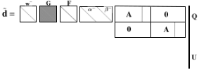 |
Figure 6: Matrix generation of simulated timestreams corresponding to Equation 33.
|
PDF / PNG |
| Pointing matrix |
 |
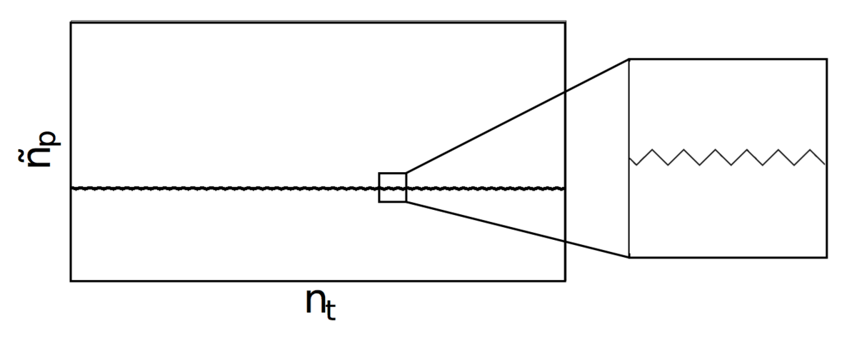
Figure 7: Pointing matrix, Λ: filled elements of the pointing matrix that transforms timestreams to an observed map in the BICEP pixelization. This matrix contains the mapping between the pointing of a single detector pair over one scanset and the output map pixels. There are 23,600 pixels in a BICEP map, denoted as ñp. There are nt filled entries, consisting of a 1 for each timestream sample. Each leg of the zigzag pattern corresponds to a halfscan within the scanset, where the telescope is scanning back and forth at a fixed elevation.
|
PDF / PNG |
| Deprojection matrix |
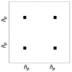 |
Figure 8: Deprojection matrix, D: filled elements of the deprojection matrix for one pair, for one phase of data. The overall dimensions are 2ñp × 2ñp, twice the number of pixels in a BICEP map.
|
PDF / PNG |
| Observation matrix |
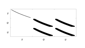 |
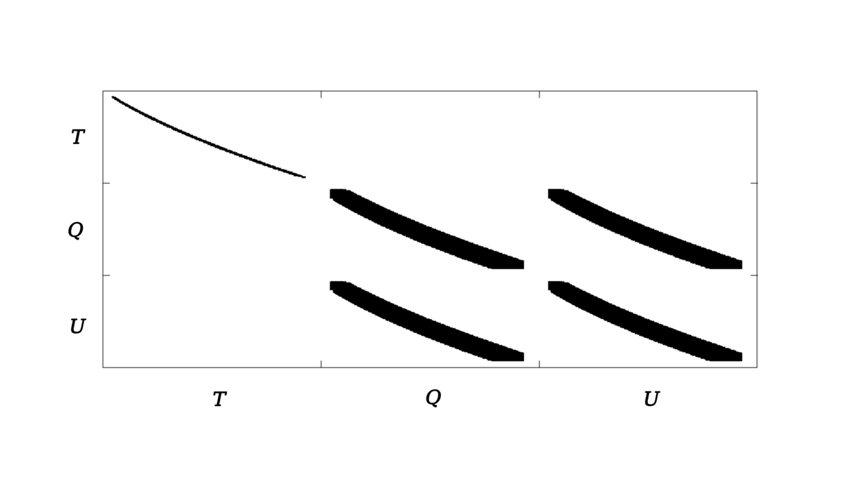
Figure 9: Observation matrix, R: filled elements of the observation matrix for the BICEP2 3 year data set. TQ, TU, UT, and QT are empty because no T→P leakage is simulated. The horizontal axis corresponds to the HEALPix pixelization and has 3 × 111,593 elements. The vertical axis corresponds to the BICEP pixelization, and has 3 × 23,600 elements. The matrix has only ∼5% of its elements filled.
|
PDF / PNG |
| Single column of the observation matrix |
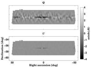 |
Figure 10: A single column of the observation matrix R, for a HEALPix Q pixel near the center of our field. The value of a single input Q pixel affects both Q and U values in the observed map over the range of declinations covered in a phase.
|
PDF / PNG |
| Comparison of Q maps |
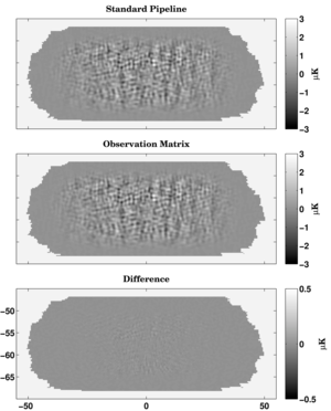 |
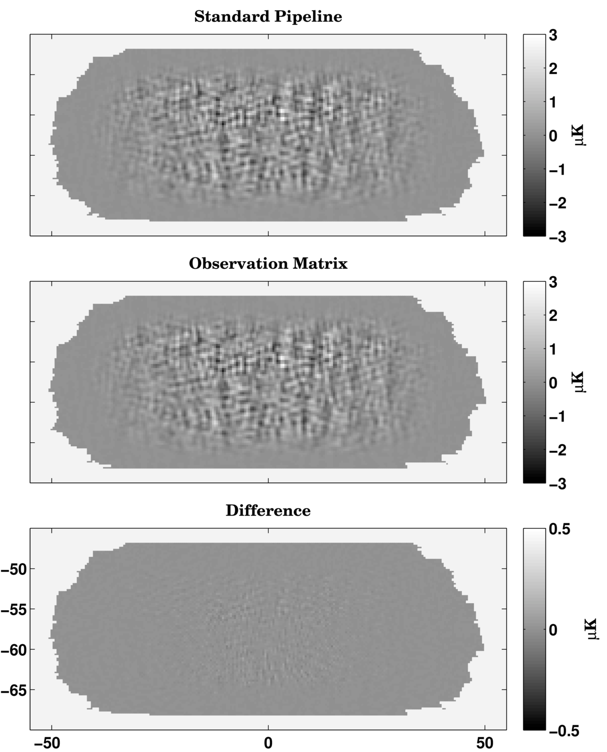
Figure 11: Comparison of observed Q maps created by the observation matrix and the standard pipeline. The input map for both is from the same simulation realization. There are small differences due to the difference in deprojection timescales, input HEALPix map resolution, and interpolation.
|
PDF / PNG |
| Comparison of power spectra |
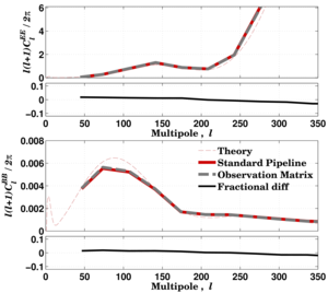 |
Figure 12: Comparison of power spectra of maps created by the observation matrix and the standard pipeline. The input map for both is from the same simulation realization, which differs from the theory curve for this particular realization in the BICEP field. The two methods are fractionally the same to within a few percent over the multipoles of interest, 50 < ℓ < 350.
|
PDF / PNG |
| Row of the observed covariance matrix |
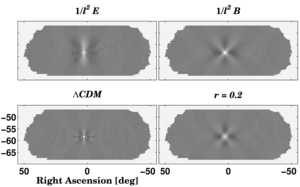 |
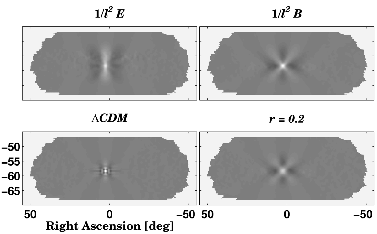
Figure 13: Maps showing a row of the observed covariance matrix C˜. The row selected corresponds to the covariance of an individual Q pixel at the center of the map. The top row shows the covariance used to calculate the pure E and B-modes described in Section 6. The bottom row shows the covariance for an input spectrum corresponding to ΛCDM [left], and r = 0.2 tensors [right].
|
PDF / PNG |
| Generalized eigenvalues |
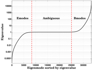 |
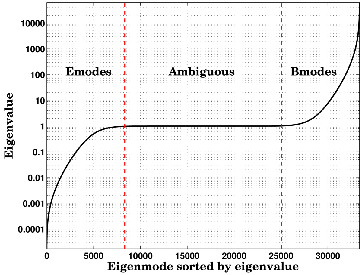
Figure 14: The generalized eigenvalues for the BICEP2 observed covariance matrix, sorted by magnitude. Eigenvalues near one correspond to ambiguous modes: the modes that are simultaneously E and B in the observed space and must be thrown out. By selecting the eigenmodes with eigenvalues that are the largest and smallest 1/4 of the set of eigenvalues (shown to the left and right of the dashed red lines), we can construct subspaces that span the spaces of B-modes and E-modes that can be effectively observed using our scan strategy and analysis.
|
PDF / PNG |
| Eigenmodes of the BICEP2 observed covariance matrix |
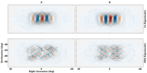 |
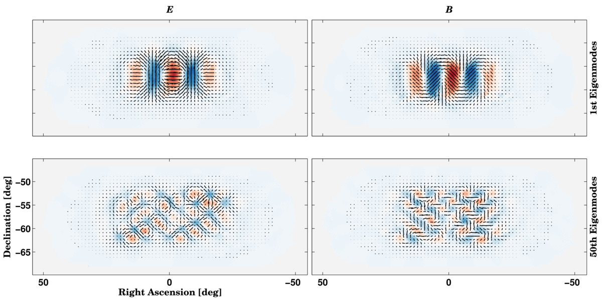
Figure 15: Eigenmodes of the BICEP2 observed covariance matrix. Shown are the modes corresponding to the largest and 50th largest eigenvalues of Equation 70. Colormap shows amplitude of E and B-modes. The eigenvalues are shown graphically in Figure 14.
|
PDF / PNG |
| E to B leakage maps |
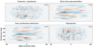 |
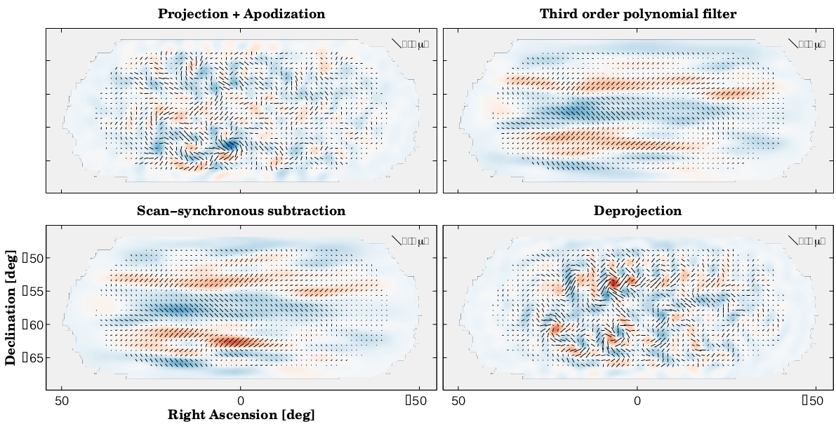
Figure 16: E to B leakage maps: examples of leaked B-modes in the BICEP2 maps. Top row, left: leaked B-modes due to map projection and apodization. Top row, right: leaked B-modes due to third order polynomial subtraction. Bottom row, left: leaked B-modes due to scan-synchronous signal subtraction. Bottom row, right: leaked B-modes due to deprojection of beam systematics.
|
PDF / PNG |
| Polarization maps showing the effectiveness of the BICEP2 purification matrix |
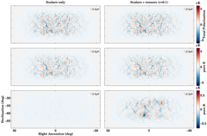 |
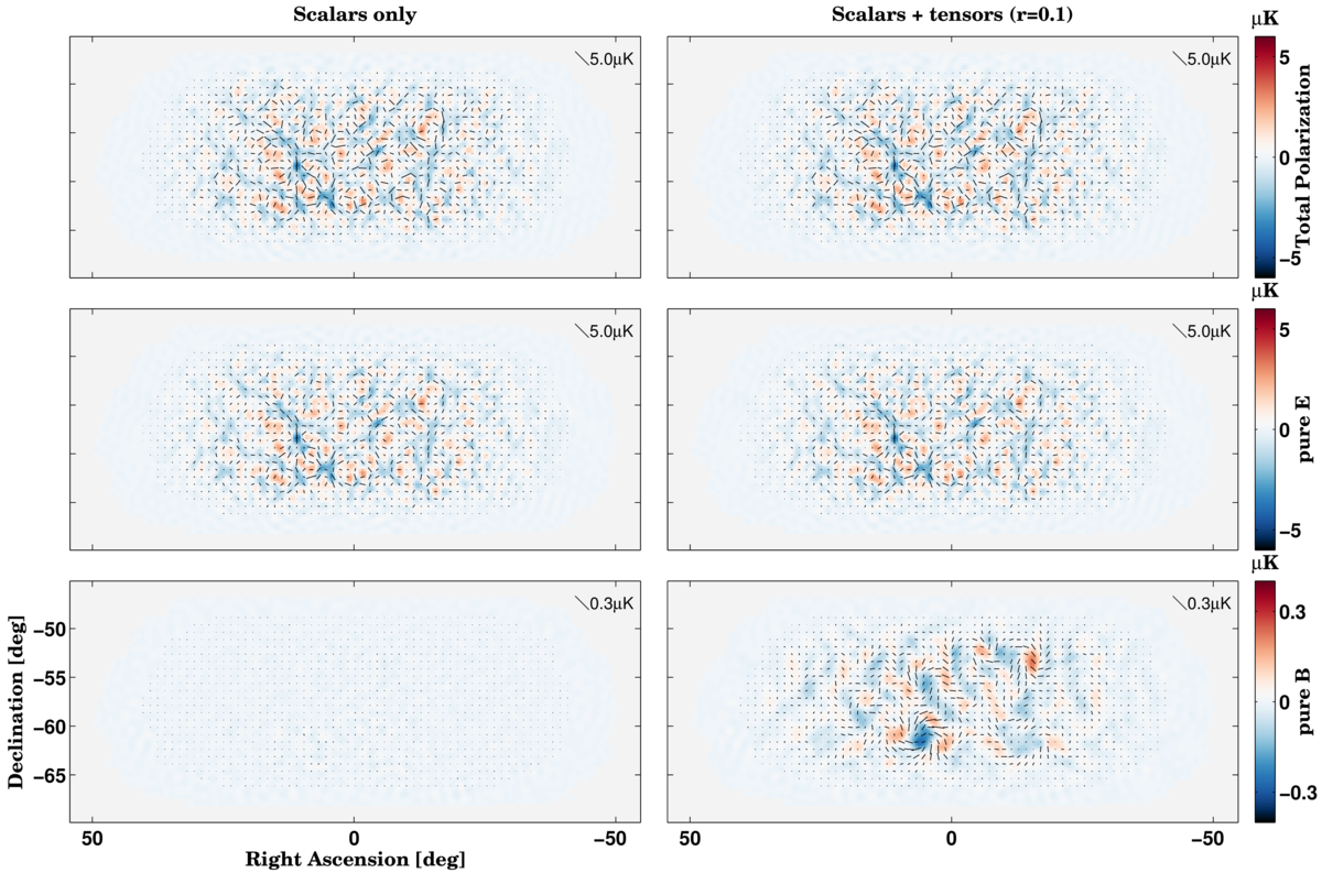
Figure 17: Polarization maps showing the effectiveness of the BICEP2 purification matrix at separating noiseless simulations into pure E and pure B. Left column: on a scalar only unlensed-ΛCDM BICEP2 simulation. Right column: on the same simulation with the addition of a small tensor component. Top row: the total polarization of the BICEP2 observed map, containing E and ambiguous modes. Center row: pure E-mode map, constructed by projecting the total polarization map onto the E eigenmodes found in Equation 70. Bottom row: pure B-mode map, constructed by projecting the total polarization map onto the B eigenmodes of Equation 70.
|
PDF / PNG |
| Effectiveness of the BICEP2 purification matrix |
 |
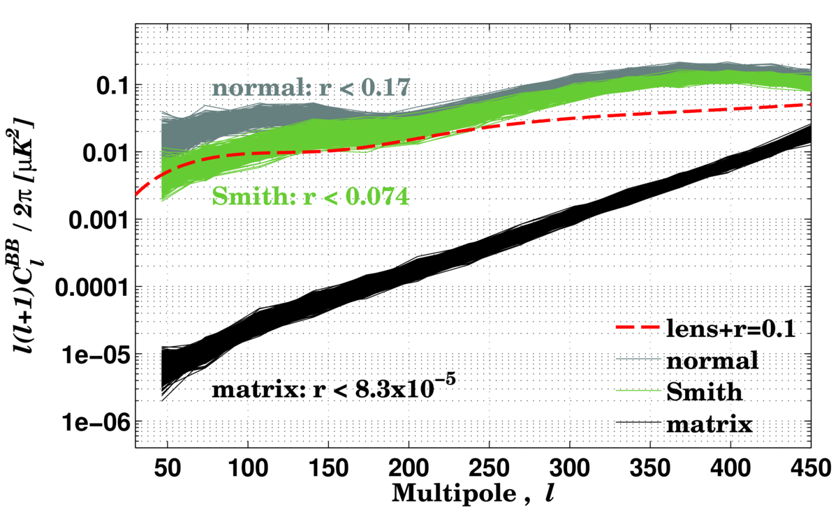
Figure 18: BB power spectra of noiseless unlensed-ΛCDM (r = 0) simulations, estimated using various methods, demonstrating the effectiveness of the BICEP2 purification matrix. The E/B leakage using the matrix estimator is 3 orders of magnitude lower than other methods.
|
PDF / PNG |
| Loss of power due to filtering, beam effects, and removal of ambiguous modes |
 |
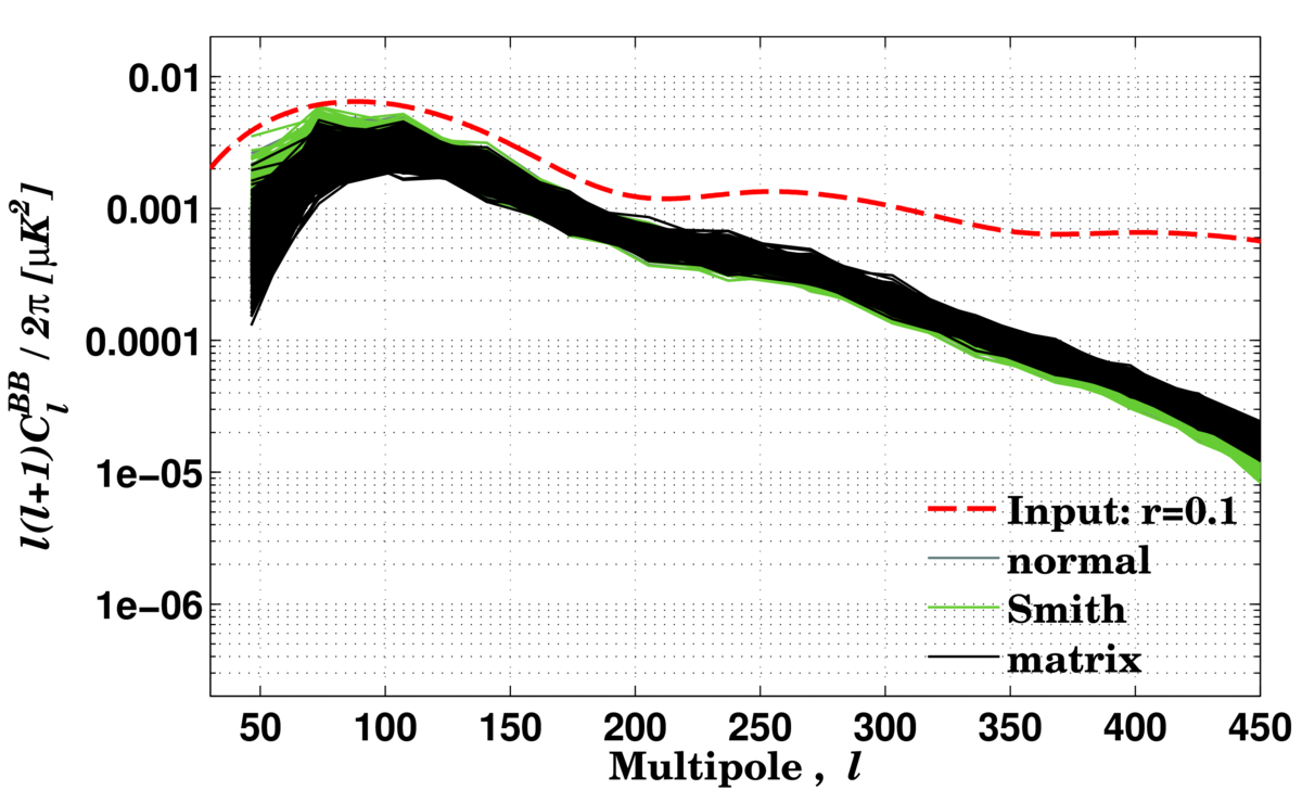
Figure 19: BB power spectra of noiseless unlensed (r = 0.1) tensor only simulations, estimated using various methods. All methods suffer from loss of power due to filtering and beam effects. The removal of ambiguous modes a low ℓ results in a further decrease in power for the matrix method. Note that the spectra in this plot have not been corrected for the beam and filter suppression factors, but in Figure 18 the correction is applied.
|
PDF / PNG |
| BB power spectra of unlensed-ΛCDM + BICEP2 noise simulations |
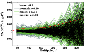 |
Figure 20: BB power spectra of unlensed-ΛCDM (r = 0) + BICEP2 noise simulations, estimated using various methods, demonstrating the effectiveness of the BICEP2 purification matrix. For BICEP2 noise levels the constraint on r (in the absense of signal) is improved by about a factor of two. (The mean of the noise and leakage have been de-biased in each case.)
|
PDF / PNG |
| Band power window functions |
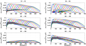 |
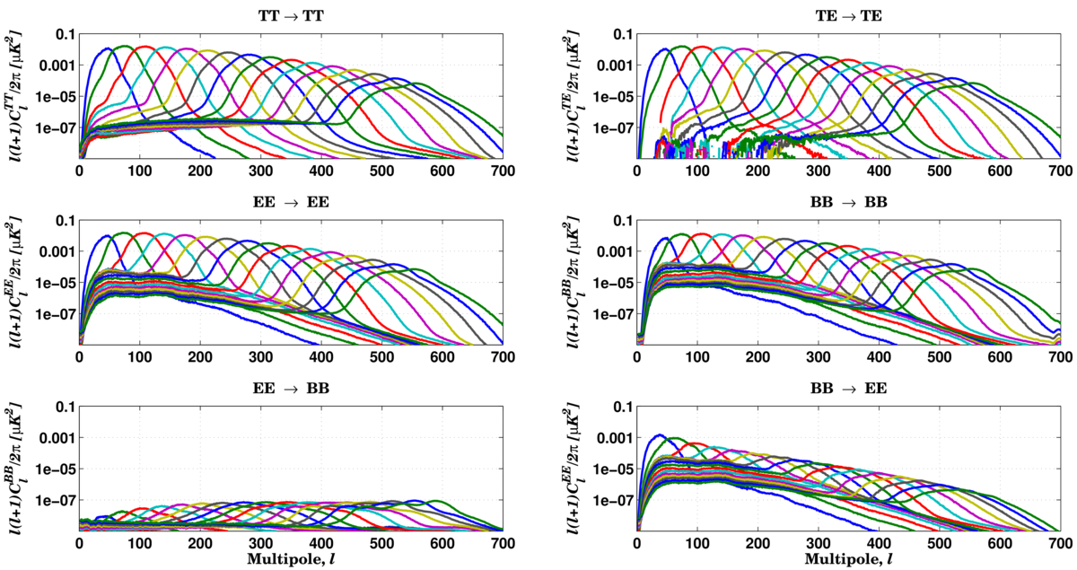
Figure 21: Band power window functions, MXXℓℓ'. Filtering causes mixing of power from low multipoles up to higher multipoles. As noted in Section 7.3.1, the BB→EE panel in the bottom right shows significantly more power since matrix purification is not applied to E-modes.
|
PDF / PNG |
| BB suppression factor |
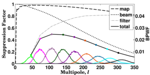 |
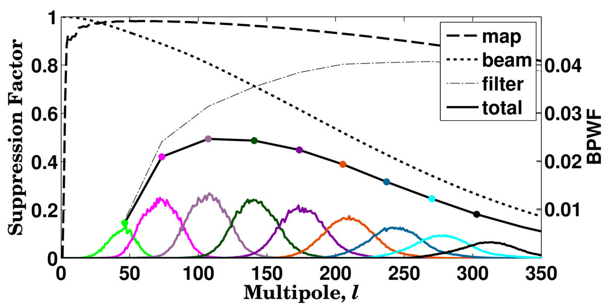
Figure 22: The BB suppression factor. At high ℓ the beam function dominates. At low ℓ the effects of filtering dominate. The map window function for the BICEP 0°.25 square pixels and finite map size is shown as a dashed line. The band power window functions are plotted in colors corresponding to individual band powers on a different scale.
|
PDF / PNG |
| Power spectra of unconstrained and constrained simulations |
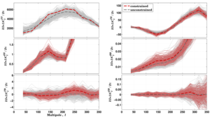 |
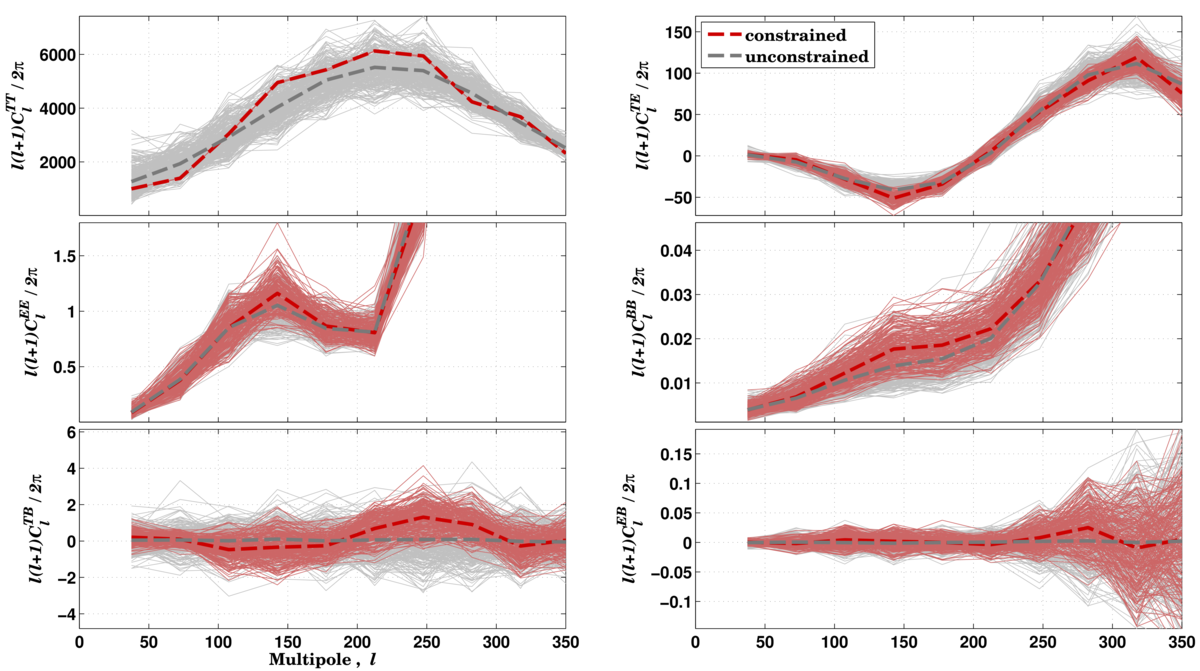
Figure 23: Power spectra of unconstrained and constrained simulations. For the constrained simulations the T sky is fixed to the Planck NILC map. By chance, the TT power in the BICEP field is above average near ℓ = 150, and this leads to increased power and variance in TE and EE for these multipoles. The BB spectrum is computed with the Smith estimator for both constrained and unconstrained simulations. It therefore contains both E/B leakage and lensing signal. The leaked B-mode power creates a significant TB signal in the constrained simulations, since the leaked B-modes correlate with the temperature template sky.
|
PDF / PNG |