| Analysis schematic |
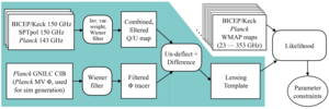 |
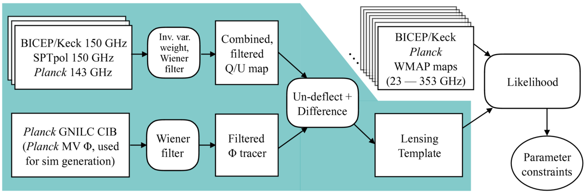
Figure 1: Schematic of the analysis flow in this work.
The rectangular blocks denote input maps; the blocks with rounded corners denote operations on maps.
The teal-colored region highlights the inputs to, and processes involved in generating, the lensing template.
The input maps include the SPTpol, BICEP/Keck, and Planck \(Q/U\) maps, the Planck GNILC CIB map, and the Planck minimum-variance (MV) reconstruction of \(\phi\).
The Planck MV \(\phi\) is in parentheses because, instead of using it as a \(\phi\) tracer, we use it to filter and normalize the CIB map and for generating simulations.
The unshaded region denotes the standard BICEP/Keck \(r\) analysis, where auto- and cross-spectra of multi-frequency maps from BICEP/Keck, Planck, and WMAP form the input data for computing likelihoods to extract parameter constraints.
The lensing template is injected into the standard analysis as an additional pseudo-frequency band.
|
PDF / PNG |
| Simulated 2D \(E\)-mode signal power spectra |
 |
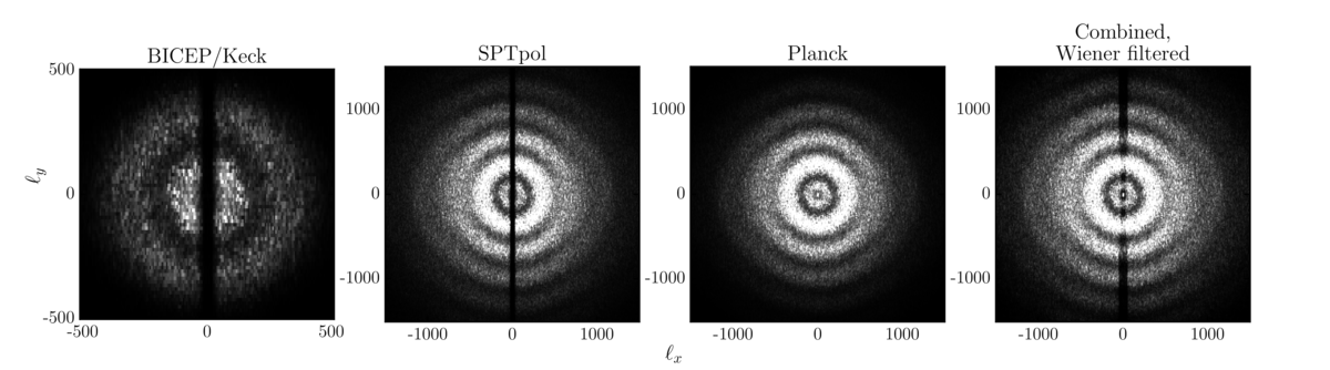
Figure 2: Simulated 2D \(E\)-mode signal power spectra of BICEP/\(Keck\), SPTpol, and \(Planck\).
The axis scales for the BICEP/\(Keck\) Fourier plane are zoomed in compared with the rest of the panels to focus on the modes accessible by BICEP/\(Keck\)’s small apertures.
The color stretch in all four panels is identical.
For BICEP/\(Keck\) and SPTpol because the observations are being made at the South Pole with scans along the azimuth direction, scan-wise filtering leads to modes along the \(\ell_y\) axis being suppressed.
These filtered modes along the \(\ell_y\) axis can be partially filled in using measurements from Planck.
To generate the combined, Wiener filtered 2D \(E\)-mode signal power spectra on the rightmost panel, the three sets of modes to the left are corrected for beam and filtering, combined using inverse-noise weighting, and Wiener filtered to suppress modes which remain noisy in the combined set (as described in Sec. III A 3).
We see that some modes remain unavailable for lensing template construction at \(\left| \ell_x \right| \lt 100\) and \(\left| \ell_y \right| \gt 500\).
|
PDF / PNG |
| \(Q/U\) maps and lensing templates |
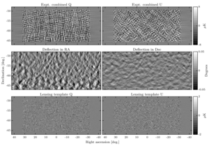 |
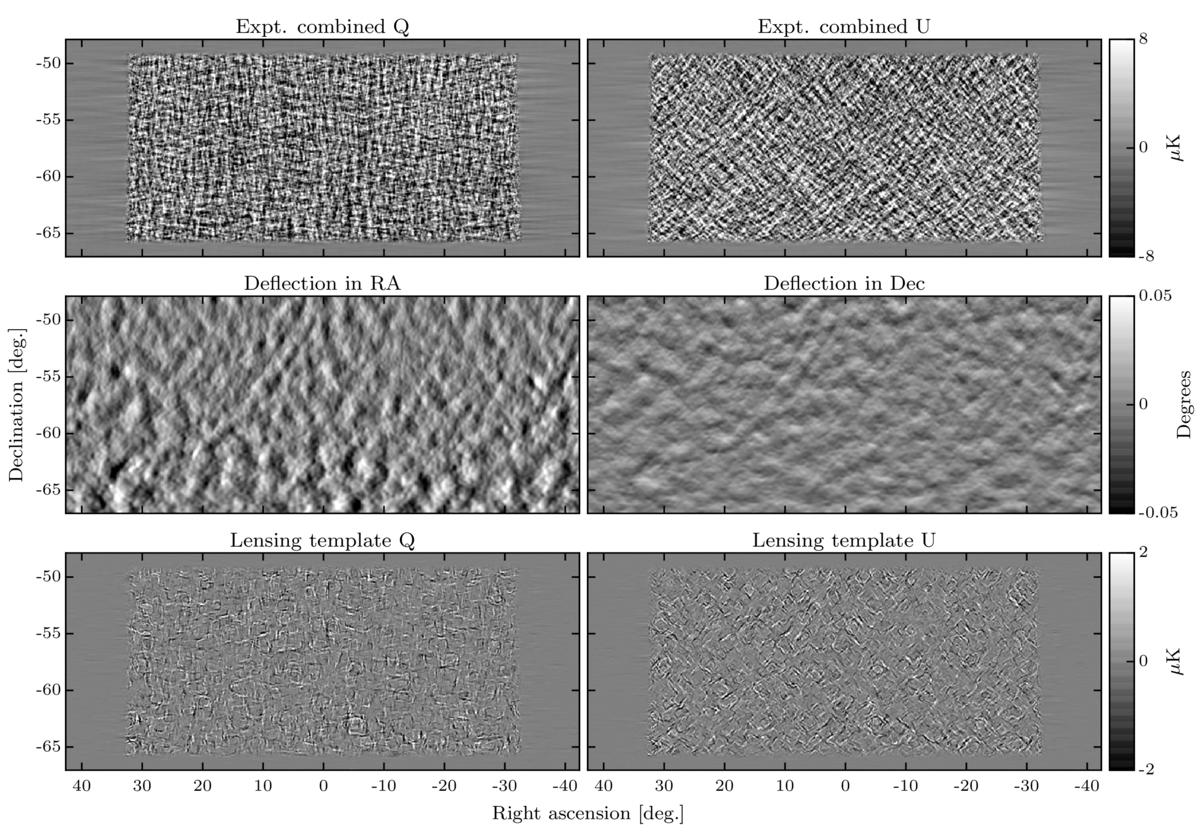
Figure 3: The top two panels show the experiment-combined and Wiener filtered \(Q/U\) maps.
The middle two panels show the \(x\) and \(y\) derivatives of the normalized and Wiener filtered \(Planck\) CIB map.
Signal and noise are approximately equal in these maps.
Due to the foreshortening effect the RA deflections are larger and increase towards more negative Dec.
The \(Q/U\) maps in the top panels are undeflected by the angles shown in the middle panels and differenced with the initial maps to form the lensing template \(Q/U\) maps shown in the bottom panels.
|
PDF / PNG |
| Sky regions |
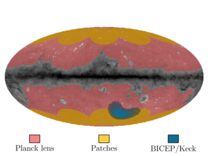 |
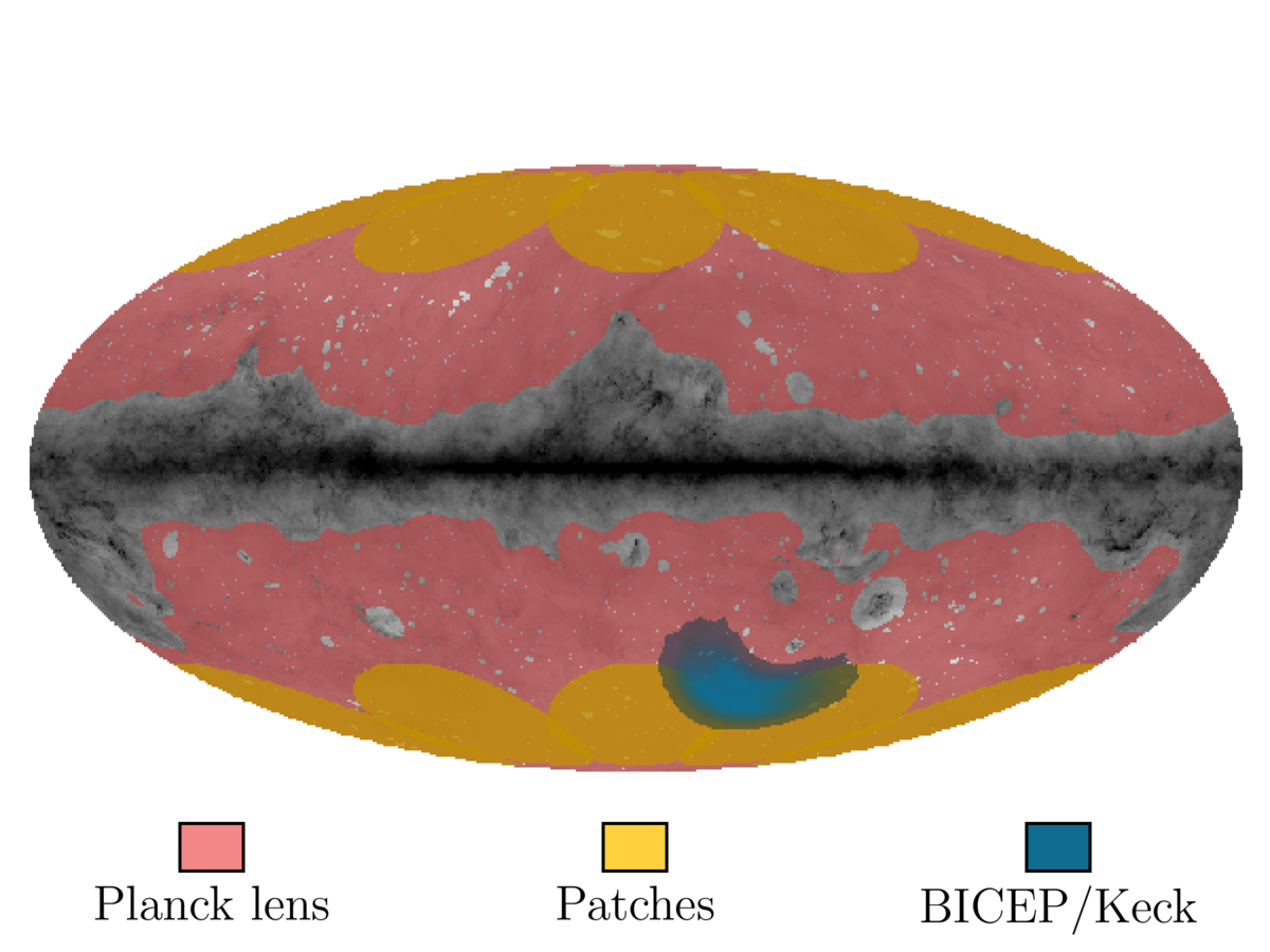
Figure 4: The light red regions denote the Planck lensing mask, used for computing the “full sky” average of GNILC CIB and \(\phi^\prime\) map cross-correlation.
The yellow regions are the eight patches with similar size and unpolarized dust amplitudes as the BICEP/Keck patch.
These patches used for measuring the mean and scatter of the CIB auto-spectra and CIB\(\times\phi^\prime\), which are used as inputs to simulating CIB and filtering the CIB map.
The overlaps between the yellow patches are small and apodization is applied when calculating the auto- and cross-spectra.
The BICEP/Keck patch is shaded in blue.
The background is the Planck dust intensity map.
|
PDF / PNG |
| Binned correlation factor |
 |
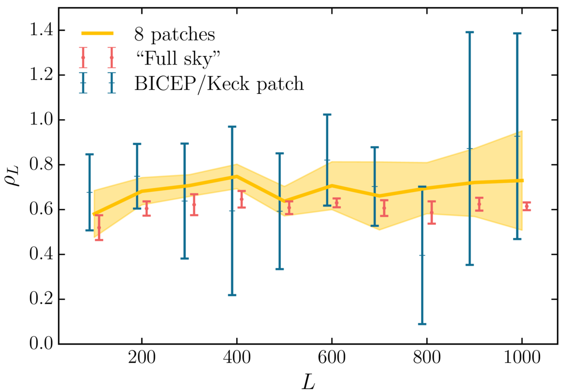
Figure 5: The binned correlation factor \(\rho_L = \mathcal{C}_L^{I\phi^\prime} / \sqrt{ \mathcal{C}_L^{II} \mathcal{C}_L^{\phi\phi} }\) for the eight patches, the full sky, and the BICEP/Keck patch.
“Full sky” corresponds to the overlap area between the Planck lensing mask and the GNILC CIB map.
The \(\rho_L\) in the BICEP/Keck patch is consistent with those measured across the eight patches.
The yellow band denoted by “8 patches” is the mean and standard deviation of \(\rho_L\) across the 8 patches.
The error bars for the red and blue points are computed by taking the standard error of \(\rho_L\) within each \(\Delta L\) = 100 bin.
The red and blue points are shifted for clarity.
|
PDF / PNG |
| Difference bandpowers between baseline and alternate analyses |
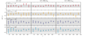 |
Figure 6: Difference bandpowers (\(\Delta \mathcal{C}_\ell\), see definition in text) between the baseline analysis and analyses with one parameter changed, and the uncertainties on those difference bandpowers, both scaled by the statistical uncertainties on the baseline analysis bandpowers.
The label at the top left hand corner of each row indicates which parameter has been modified and how it is modified.
The left to right columns show the difference bandpowers from the lensing template auto-spectrum, lensing template cross-spectrum with the BK14 95 GHz map, and lensing template cross-spectrum with the BK14 150 GHz map.
The gray bands indicate the \(0.5\sigma\) statistical uncertainty of the baseline spectra.
The \(\chi_\mathrm{sys}^2\) and PTE of the difference bandpowers are listed in Table I.
We find the data difference bandpowers to be consistent with the spread in the simulation difference bandpowers.
|
PDF / PNG |
| \(BB\) auto- and cross-spectra |
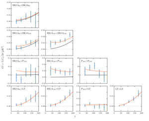 |
Figure 7: \(BB\) auto- and cross-spectra calculated using BICEP2/Keck 95 & 150 GHz maps, the Planck 353 GHz map, and the lensing template developed in this paper.
The black lines show the model expectation values for lensed-ΛCDM, while the red lines show the expectation values of the baseline lensed-ΛCDM+dust model from the BK14 analysis (\(r = 0\), \(A_d = 4.3 \, \mu K^2\), \(\beta_d = 1.6\), \(\alpha_d = −0.4\)), and the error bars are scaled to that model.
Compared to the BK14 BB spectra, which contain both foregrounds and lensing components, the lensing template represents an alternate way to estimate the lensing B-modes which is largely foreground-immune, and, as we see here, provides good signal-to-noise in the resulting auto- and cross-spectra.
|
PDF / PNG |
| Histograms of maximum-likelihood values of \(r\), \(A_d\), and \(A_\mathrm{sync}\) |
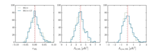 |
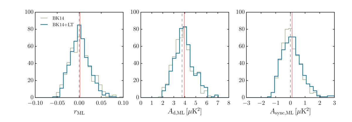
Figure 8: Histograms of maximum-likelihood values of \(r\), \(A_d\), and \(A_\mathrm{sync}\) from 499 realizations of BK14+LT (blue) and BK14 (gray) lensed-ΛCDM+dust+noise simulations in the baseline model with 6 free parameters: \(r\), \(A_d\), \(A_\mathrm{sync}\), \(\beta_d\), \(\beta_s\) and \(\alpha_d\).
The red lines mark the means of the distributions for the BK14+LT simulation set and the gray dashed lines mark the input values.
\(\sigma(r)\) from the BK14+LT (BK14) simulation set is 0.022 (0.024) from the leftmost panel.
|
PDF / PNG |
| Posterior distributions given the BK14+LT data set |
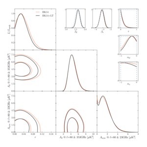 |
Figure 9: Posterior distributions of the baseline model parameters given the BK14+LT data set (black lines) compared with the BK14 data set (red lines, which are the same as the black lines in Fig. 4 of the BK14 paper).
The lensing template is constructed using combined \(Q/U\) maps from SPTpol, BICEP/Keck, and Planck (Sec. III A 3) and a CIB map as the \(\phi\) tracer (Sec. III B 1).
The 95% C.L. upper limit on the tensor-to-scalar ratio tightens from \(r_{0.05} \lt 0.090\) to \(r_{0.05} \lt 0.082\) with the addition of the lensing template.
The parameters \(A_d\) and \(A_\mathrm{sync}\) are the amplitudes of the dust and synchrotron \(B\)-mode spectra, where \(\beta\) and \(\alpha\) are the frequency and spatial spectral indices respectively.
The dust-synchrotron correlation parameter is denoted by \(\epsilon\).
The up-turn of the 1D posterior distribution of \(A_\mathrm{sync}\) as it approaches zero comes from the increased volume allowed by the \(\epsilon\) parameter as \(\epsilon\) becomes ambiguous when \(A_\mathrm{sync} = 0\).
In the 1D panels for the \(\alpha\), \(\beta\), and \(\epsilon\) parameters, the blue dashed lines denote the priors for each parameter.
|
PDF / PNG |
| Posterior distributions on \(r\) and \(A_L\) |
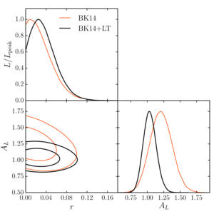 |
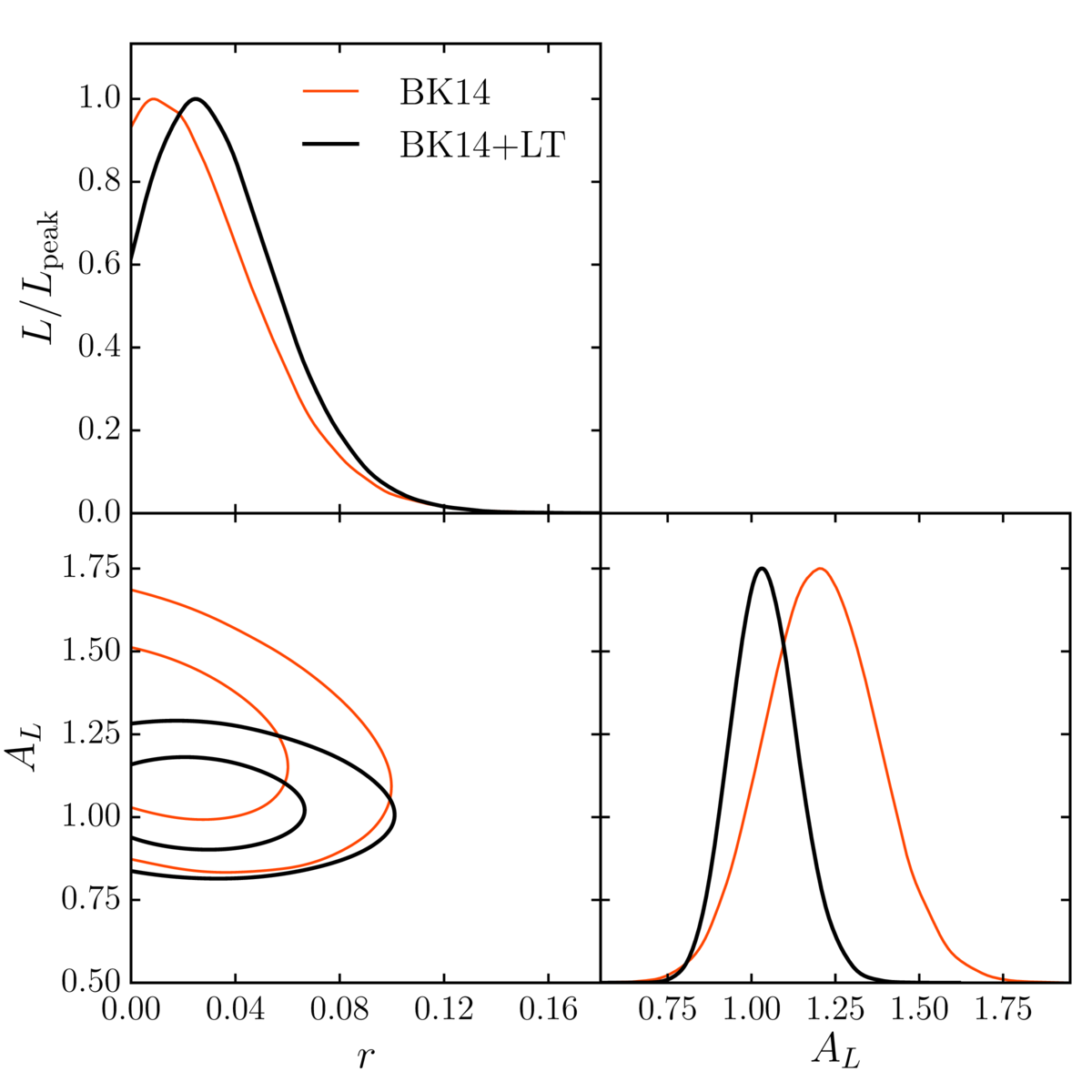
Figure 10: Posterior distributions on \(r\) and \(A_L\), a parameter used to scale the lensing \(BB\) power, from an alternative analysis in which the amplitude of lensing is a free parameter.
With the addition of the lensing template, the probability of shuffling lensing power to other parameters is reduced, thus the degeneracy between \(r\) and \(A_L\) is reduced.
|
PDF / PNG |
| \(r\) posteriors with alternate lensing templates |
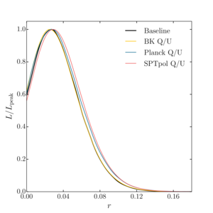 |
Figure 11: The \(r\) posterior curves from the baseline analysis, along with \(r\) curves from analyses using lensing templates constructed from \(Q/U\) maps from only one of the three experiments: BICEP/Keck, Planck, and SPTpol.
The shifts in the curves are consistent with expectations from simulations.
|
PDF / PNG |