| T, Q, and U maps |
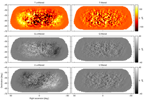 |
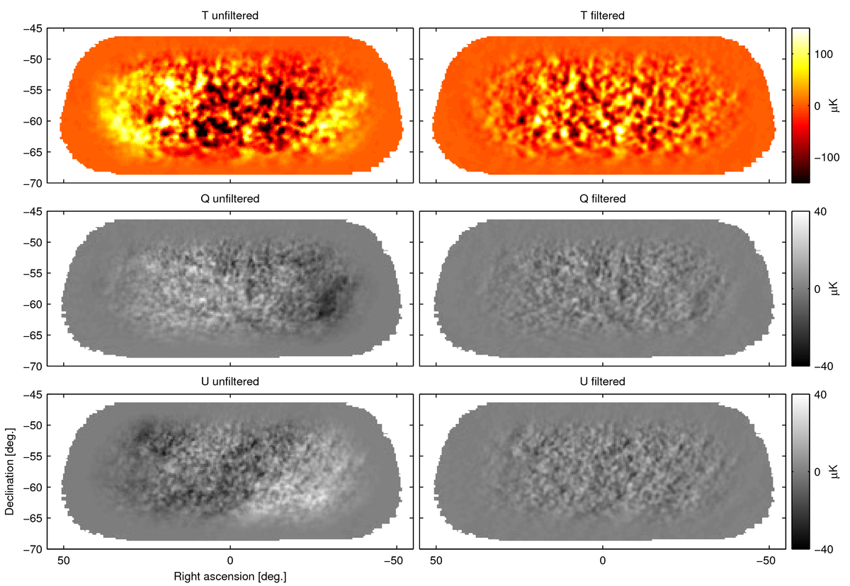
Figure 1: Planck 353 GHz T, Q, and U maps before
(left) and after (right) the application of BICEP2/Keck filtering.
In both cases the maps have been multiplied by the BICEP2/Keck
apodization mask.
The Planck maps are presmoothed to the BICEP2/Keck
beam profile and have the mean value subtracted.
The filtering, in particular the third order polynominal subtraction
to suppress atmospheric pickup, removes large-angular scale signal along the
BICEP2/Keck scanning direction (parallel to the right ascension
direction in the maps here).
|
PDF / PNG |
| Spectra between BICEP2/Keck maps at 150 GHz and Planck maps at 353 GHz |
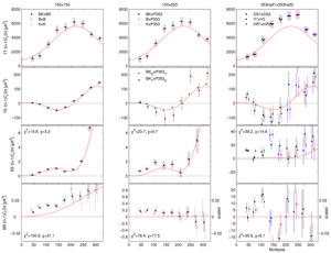 |
Figure 2: Single- and cross-frequency spectra between BICEP2/Keck
maps at 150 GHz and Planck maps at 353 GHz.
The red curves show the lensed-ΛCDM expectations.
The left column shows single-frequency spectra of the
BICEP2, Keck Array, and combined BICEP2/Keck maps.
The BICEP2 spectra are identical to those in BK-I,
while the Keck Array and combined are as given in
BK-V.
The center column shows cross-frequency spectra between BICEP2/Keck
maps and Planck 353 GHz maps.
The right column shows Planck 353 GHz data-split cross-spectra.
In all cases the error bars are the standard deviations of
lensed-ΛCDM+noise simulations and hence contain no sample
variance on any other component.
For EE and BB the χ2 and χ (sum of deviations)
versus lensed-ΛCDM for the nine bandpowers shown is marked at upper and lower left
(for the combined BICEP2/Keck points and DS1×DS2, respectively).
In the bottom row (for BB) the center and right panels have a scaling applied such
that signal from dust with the fiducial frequency spectrum
would produce signal with the same apparent amplitude as in the 150 GHz
panel on the left (as indicated by the right-side y-axes).
We see from the significant excess apparent in the bottom center panel
that a substantial amount of the signal detected
at 150 GHz by BICEP2 and Keck Array indeed appears to be
due to dust.
|
PDF / PNG |
| EE and BB cross-spectra |
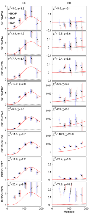 |
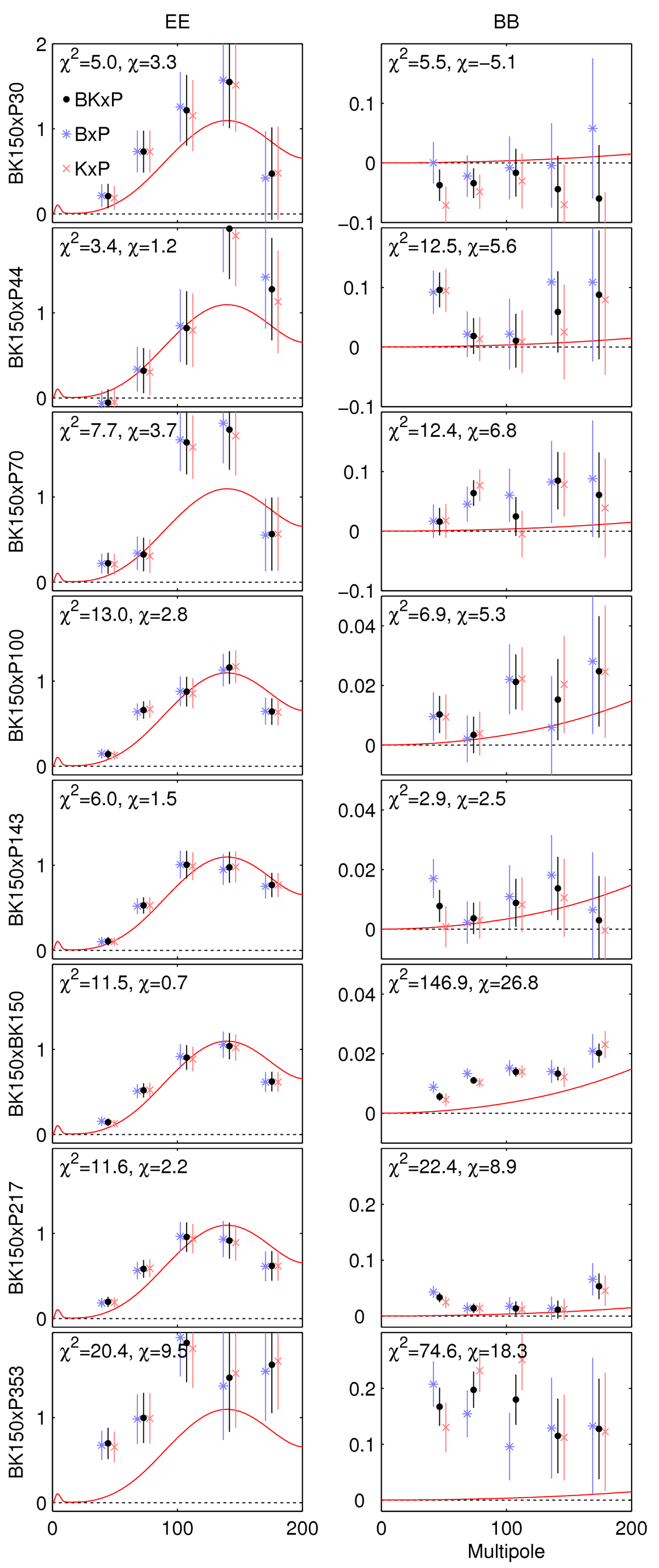
Figure 3: EE (left column) and BB (right column) cross-spectra between
BICEP2/Keck maps and all of the polarized frequencies of Planck.
In all cases the quantity plotted is ℓ(ℓ+1)Cℓ/2π
in units of μKCMB2, and the red curves show the lensed-ΛCDM expectations. The error bars are the standard deviations of
lensed-ΛCDM+noise simulations and hence contain no sample
variance on any other component.
Also note that the y-axis scales differ from panel to panel
in the right column.
The χ2 and χ (sum of deviations)
versus lensed-ΛCDM for the five bandpowers shown
is marked at upper left.
There are no additional strong detections of
deviation from lensed-ΛCDM over those
already shown in Figure 2
although BK150×P217 shows some evidence
of excess.
|
PDF / PNG |
| Differences between BICEP2 and Keck Array cross-spectra with Planck |
 |
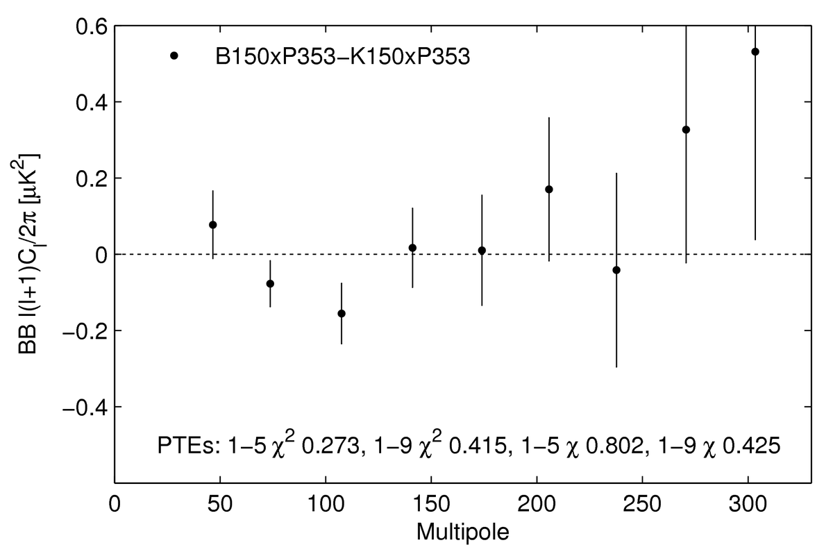
Figure 4: Differences of B150×P353 and K150×P353 BB cross-spectra.
The error bars are the standard deviations of the pairwise
differences of signal+noise simulations that share common
input skies.
The probability to exceed the observed values of χ2
and χ statistics, as evaluated against the simulations,
is quoted for bandpower ranges 1–5 (20<ℓ<200) and 1–9 (20<ℓ<330).
There is no evidence that these spectra are statistically incompatible.
|
PDF / PNG |
| Differences between the standard power spectrum estimator and alternate
estimators |
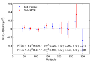 |
Figure 5: Differences of B150×P353 BB cross-spectra
from the standard power spectrum estimator and alternate
estimators.
The error bars are the standard deviations of the pairwise
differences of signal+noise simulations that share common
input skies.
The probability to exceed the observed values of χ2 and
χ statistics, as evaluated against simulations, is quoted for bandpower
ranges 1–5 (20<ℓ<200) and 1–9 (20<ℓ<330).
We see that the differences of the real spectra are consistent
with the differences of the simulations.
|
PDF / PNG |
| Likelihood results from a lensed-ΛCDM+r+dust model
|
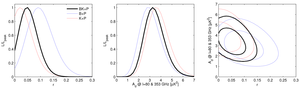 |
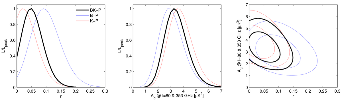
Figure 6: Likelihood results from a basic lensed-ΛCDM+r+dust
model, fitting BB auto- and cross-spectra taken between
maps at 150 GHz, 217, and 353 GHz.
The 217 and 353 GHz maps come from Planck.
The primary results (heavy black) use the 150 GHz
combined maps from BICEP2/Keck.
Alternate curves (light blue and red) show how
the results vary when the BICEP2 and Keck Array
only maps are used.
In all cases a Gaussian prior is placed on the dust frequency
spectrum parameter βd = 1.59±0.11.
In the right panel the two dimensional contours
enclose 68% and 95% of the total likelihood.
|
PDF / PNG |
| Likelihood results when varying the data sets and model priors |
 |
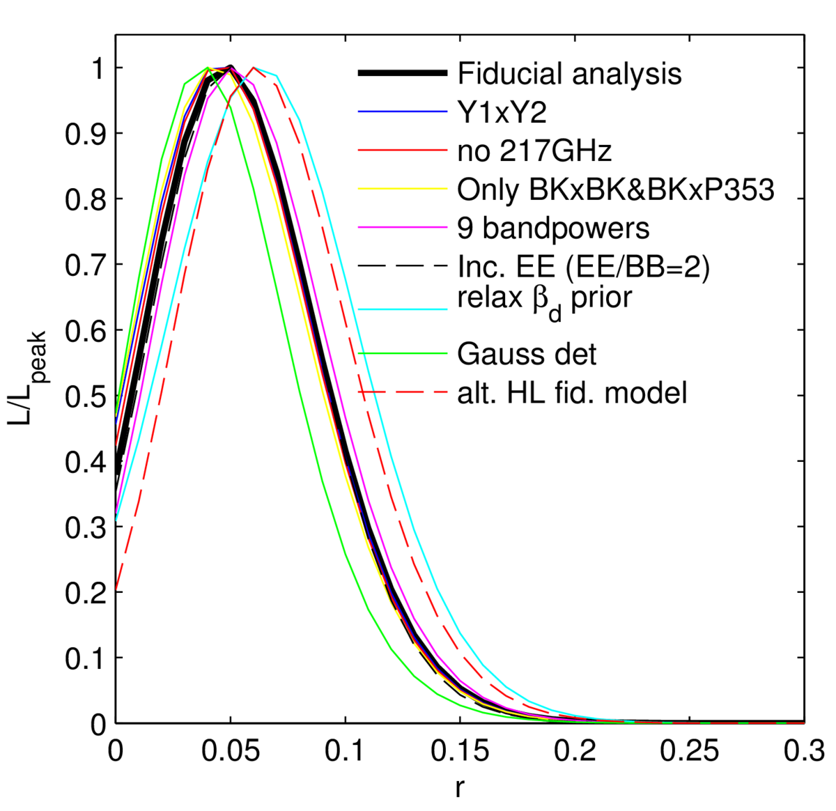
Figure 7: Likelihood results when varying the data sets
used and the model priors.
|
PDF / PNG |
| Likelihood results including synchrotron |
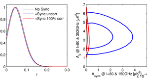 |
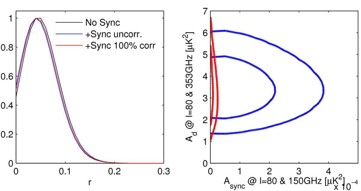
Figure 8:
Likelihood results for a fit when adding the lower frequency
bands of Planck, and extending the model to include a
synchrotron component.
The results for two different assumed degrees of
correlation between the dust and synchrotron sky patterns
are compared to those for the comparable model
without synchrotron.
|
PDF / PNG |
| Likelihood results allowing AL to vary |
 |
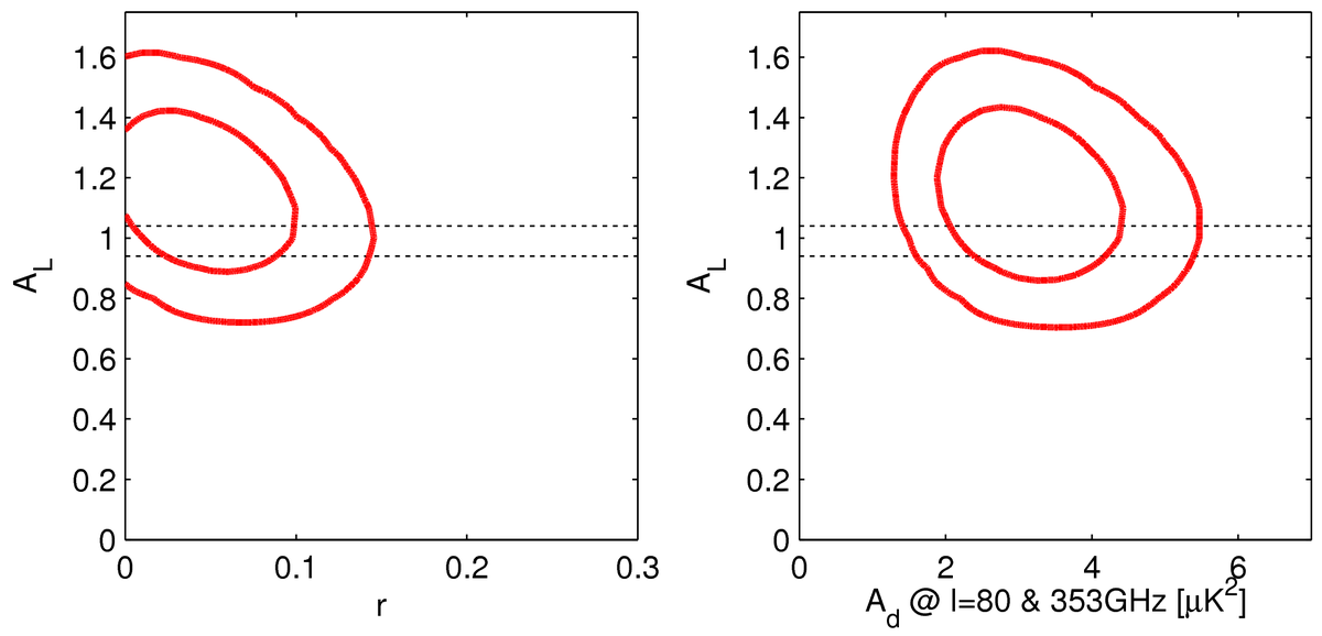
Figure 9:
Likelihood results for a fit allowing the lensing
scale factor AL to float freely and using all nine bandpowers.
Marginalizing over r and Ad, we find that
AL=1.13±0.18 and AL=0 is
ruled out with 7.0 σ significance.
|
PDF / PNG |
| Likelihood results from simulations |
 |
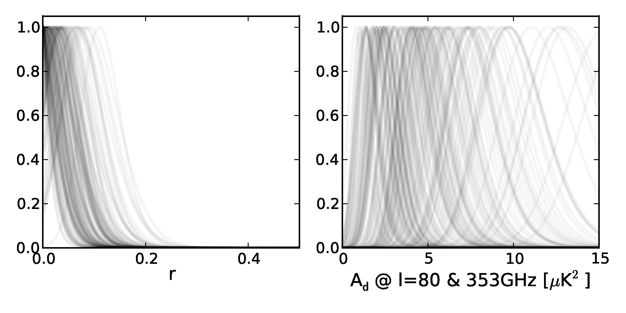
Figure 10:
Likelihoods for r and Ad, using BICEP2/Keck and
Planck,
as plotted in Figure 6, overplotted on
constraints obtained from realizations of a
lensed-ΛCDM+noise+dust model with dust power
similar to that favored by the real data (Ad=3.6 μK2).
Half of the r curves peak at zero as expected.
|
PDF / PNG |
| Likelihood results from Planck Sky Model simulations |
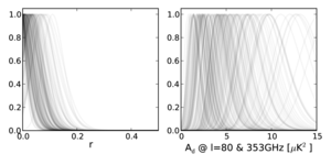 |
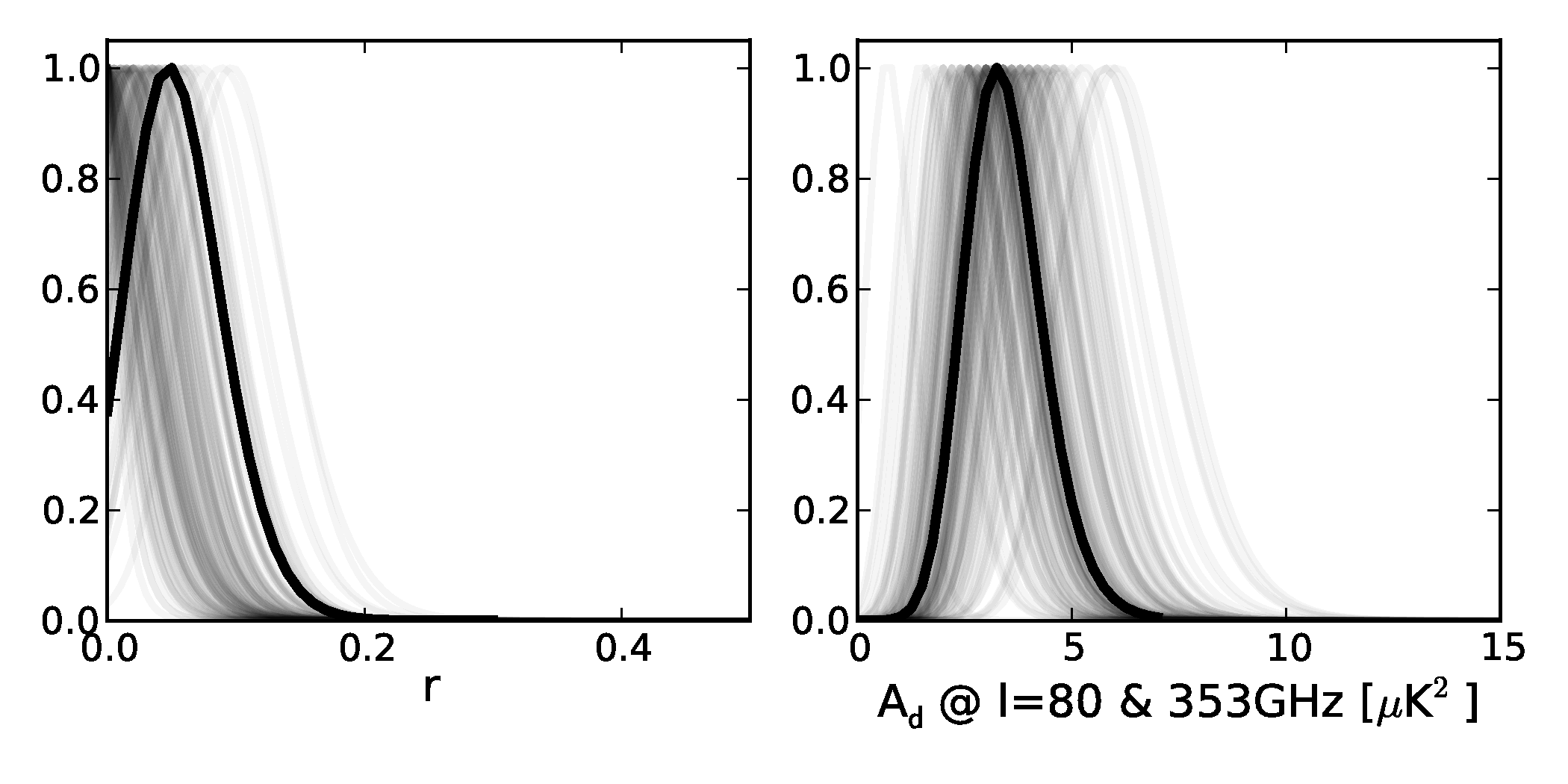
Figure 11:
Constraints obtained when adding dust realizations
from the Planck Sky Model version 1.7.8 to the base
lensed-ΛCDM+noise simulations.
(Curves for 139 regions with peak Ad<20 μK2
are plotted.)
We see that the results for r are unbiased in the presence
of dust realizations which do not necessarily follow the
ℓ-0.42 power law or have Gaussian fluctuations about it.
|
PDF / PNG |
| BB spectrum before and after dust subtraction and Constraint on r from cleaned spectrum |
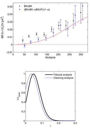 |
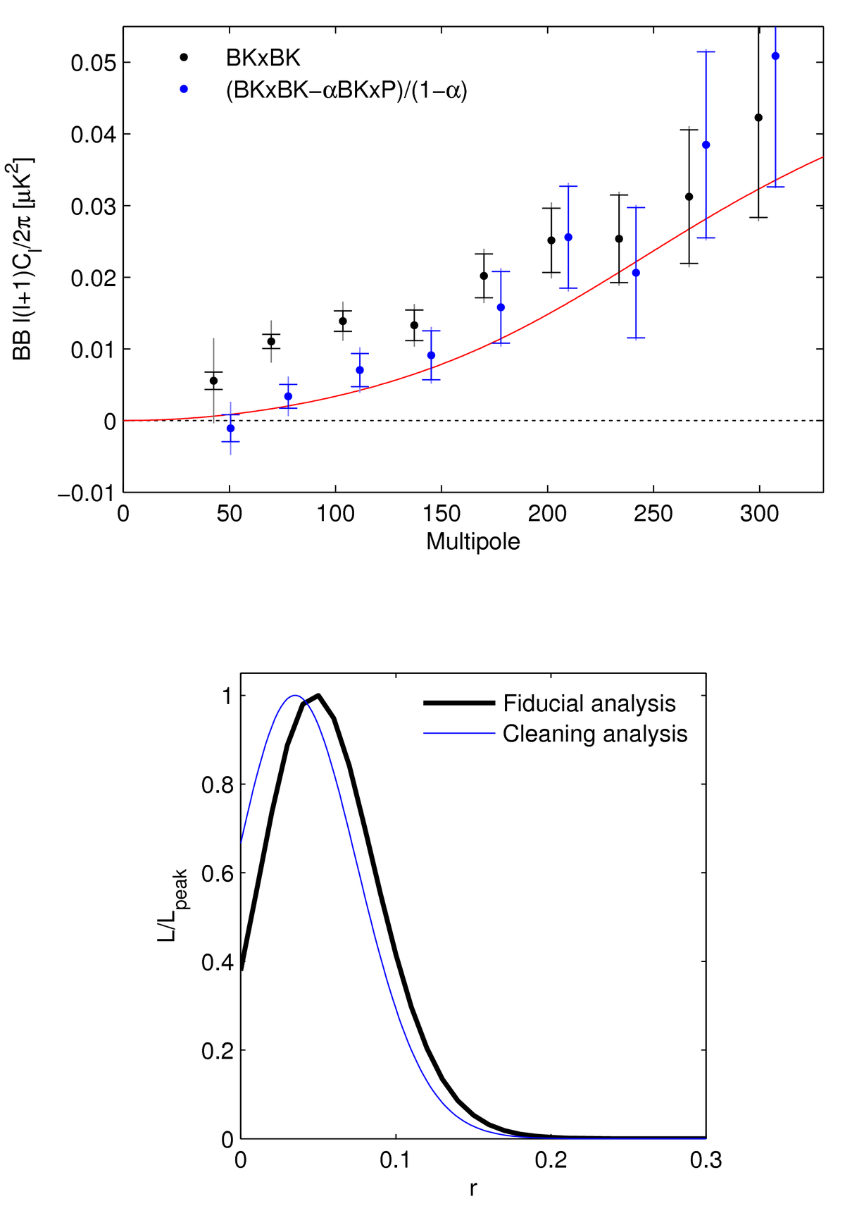
Figure 12: Upper: BB spectrum of the BICEP2/Keck maps
before and after subtraction of the dust contribution, estimated from
the cross-spectrum with Planck 353 GHz.
The error bars are the standard deviations of
simulations, which, in the latter case, have been scaled and combined
in the same way.
The inner error bars are from lensed-ΛCDM+noise simulations
as in the previous plots, while the outer error bars are from the
lensed-ΛCDM+noise+dust simulations.
The red curve shows the lensed-ΛCDM expectation.
Lower: Constraint on r derived from the cleaned spectrum
compared to the fiducial analysis shown in Figure 6.
|
PDF / PNG |
| Expectation values and uncertainties for BB in the BICEP2/Keck field |
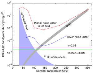 |
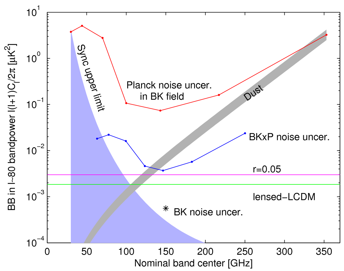
Figure 13:
Expectation values, and uncertainties thereon, for the ℓ~80
BB bandpower in the BICEP2/Keck field.
The green and magenta lines correspond to the expected signal power of
lensed-ΛCDM and r=0.05.
Since CMB units are used, the levels corresponding
to these are flat with frequency.
The grey band shows the best fit
dust model and
the blue shaded region shows the allowed region for synchrotron.
The BICEP2/Keck noise uncertainty is shown as a single starred
point, and the noise uncertainties of the Planck single-frequency
spectra evaluated in the BICEP2/Keck field are shown in red.
The blue points show the noise uncertainty of the
cross-spectra taken between BICEP2/Keck and,
from left to right, Planck 30, 44, 70, 100, 143, 217 and 353 GHz,
and plotted at horizontal positions such that they
can be compared vertically with the dust and sync curves.
|
PDF / PNG |