-
BK-XVII: Line of Sight Distortion Analysis: Estimates of Gravitational Lensing, Anisotropic Cosmic Birefringence, Patchy Reionization, and Systematic Errors
The BICEP/Keck Collaboration, ApJ 949, 43, 2023
| Figures | Download Bundle | ||
|---|---|---|---|
| Distortion field power spectra pipeline verification for polarization rotation field | 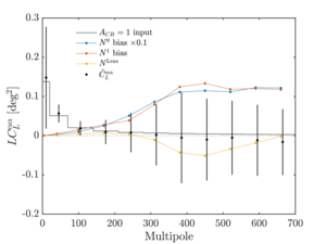 |
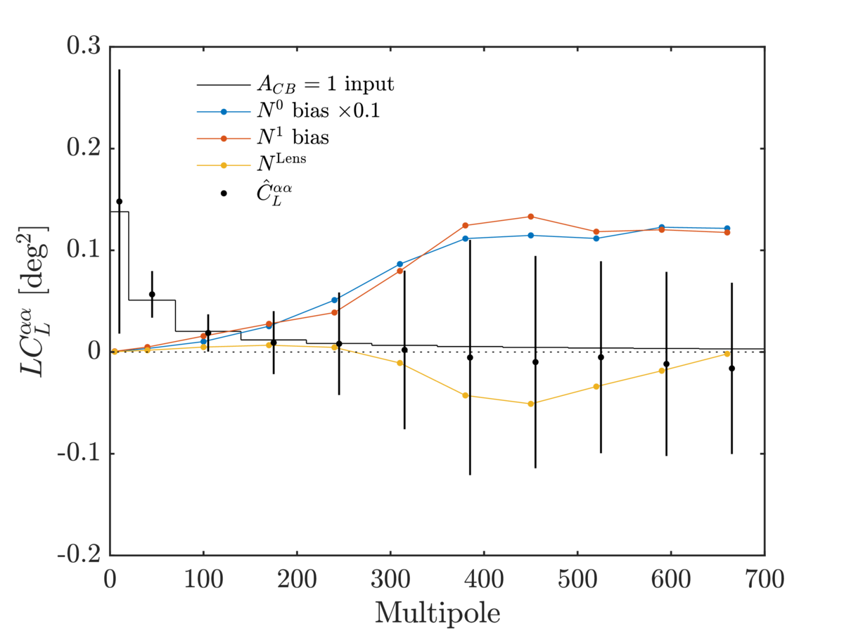
Figure 1: Example of the distortion field power spectra pipeline verification for the polarization rotation field \(\alpha(\mathbf{\hat{n}})\). The horizontal lines show the binned theory input for an \(A_{CB}=1\) spectrum. The \(\hat{C}_L^{\alpha\alpha}\), the mean simulation bandpowers, matches the input spectrum after accounting for \(N^0\), \(N^1\), and the lensing bias \(N^\mathrm{Lens}\). The error bars show the standard deviation of the simulation realizations. | PDF / PNG |
| \(E\) and \(B\) combinations for lensing convergence spectrum estimator | 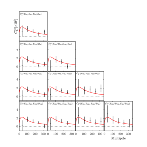 |
Figure 2: The 10 different ways to combine two sets of \(E\) and \(B\) maps to form the lensing convergence spectrum estimator \(\hat{C}_L^{\alpha\alpha}\). The red line is the theoretical lensing convergence spectrum corresponding to our fiducial model assuming Planck 2013 cosmological parameters (Planck Collaboration 2014). The top left subplot is the auto-spectrum from 95 GHz, while the bottom right subplot is the auto-spectrum from 150 GHz. The other subplots contain information from both 95 and 150 GHz. We examine the 10 spectra individually, all 10 spectra combined, and some other data combinations and find that they are all consistent with the lensed ΛCDM predictions. | PDF / PNG |
| Lensing convergence power spectrum | 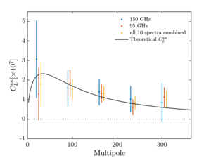 |
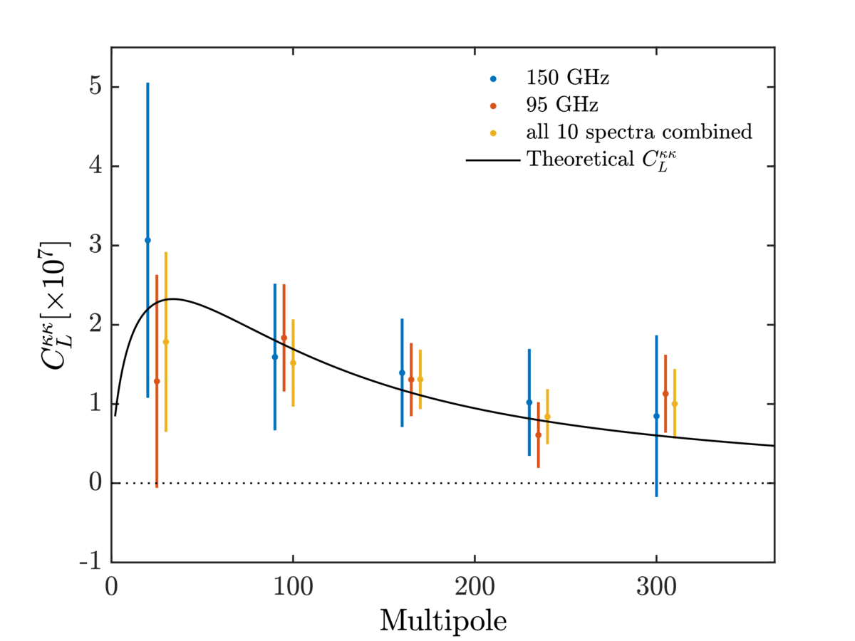
Figure 3: Lensing convergence power spectrum \(C_L^{\alpha\alpha}\) for the 95 GHz autospectrum, the 150 GHz auto-spectrum, and all 10 auto- and cross-spectra combined. | PDF / PNG |
| Comparison of lensing amplitude constraints |  |
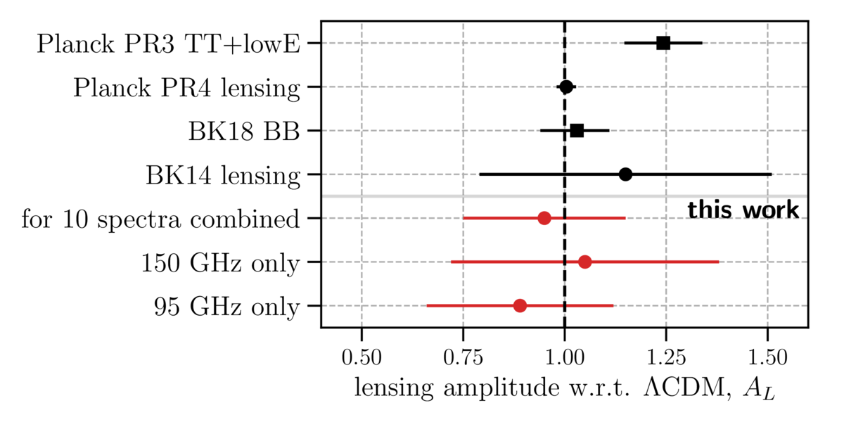
Figure 4: Comparison of the constraints of this paper with the latest constraints of the lensing amplitude \(A_L\) from the Planck PR3 temperature power spectrum, TT+lowE (Planck Collaboration 2020); the Planck PR4 lensing reconstruction (Carron et al. 2022); the BK18 B-mode power spectrum measurement (BK–XIII) using the same data set; and the previous measurement from the lensing potential reconstruction using BK14 data (BK–VIII). Bullet points denote constraints from the lensing potential auto-power spectrum, and squares are used for measurements using CMB two-point functions. | PDF / PNG |
| Power spectra of patchy reionization | 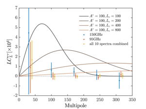 |
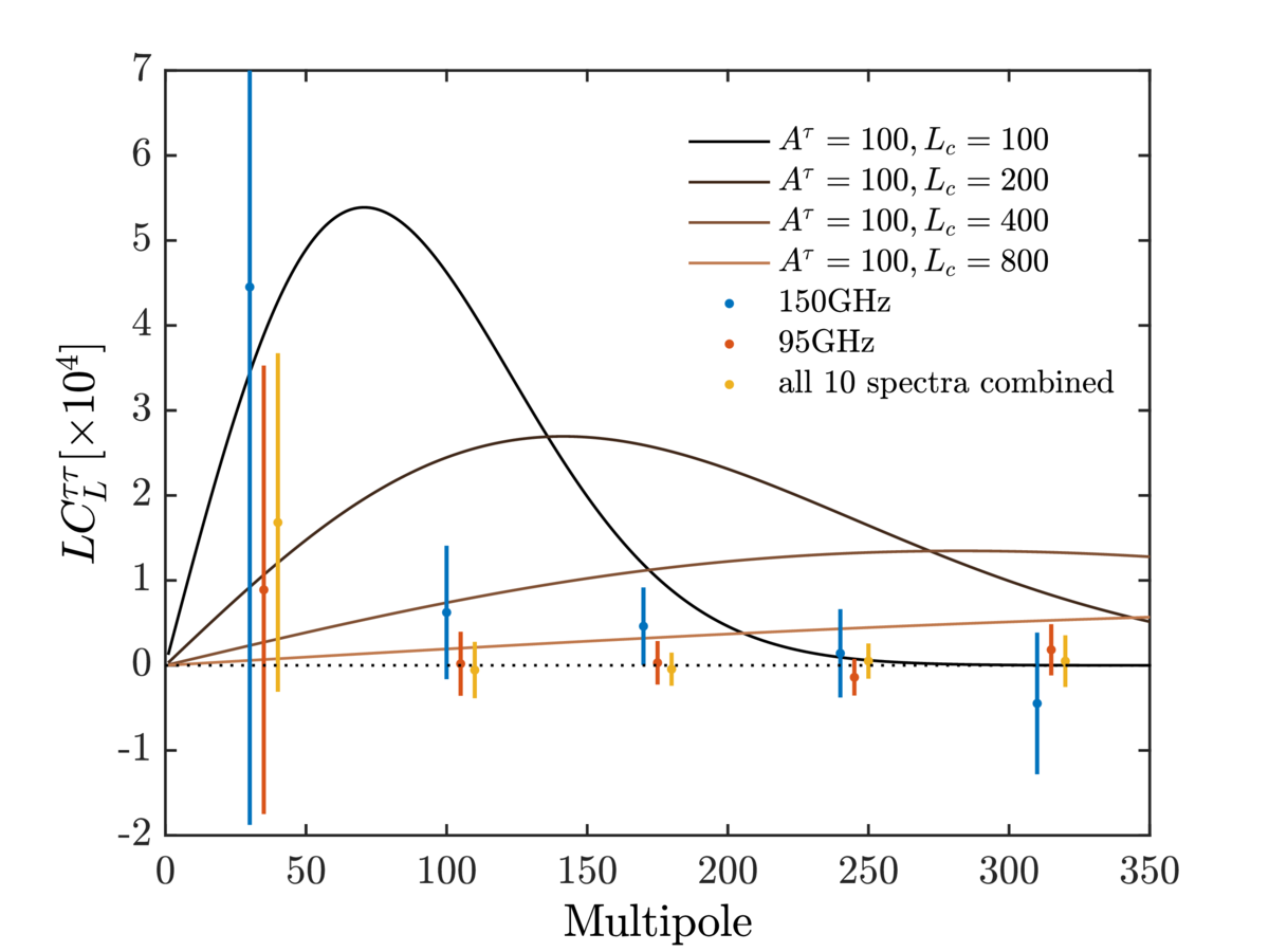
Figure 5: Data and model power spectra of patchy reionization. The solid lines show fiducial model spectra from Equation (6) for \(L_c\) = 100, 200, 400, and 800. The data points show \(\hat{C}_L^{TT}\) for 150 GHz only, 95 GHz only, and all 10 spectra combined. | PDF / PNG |
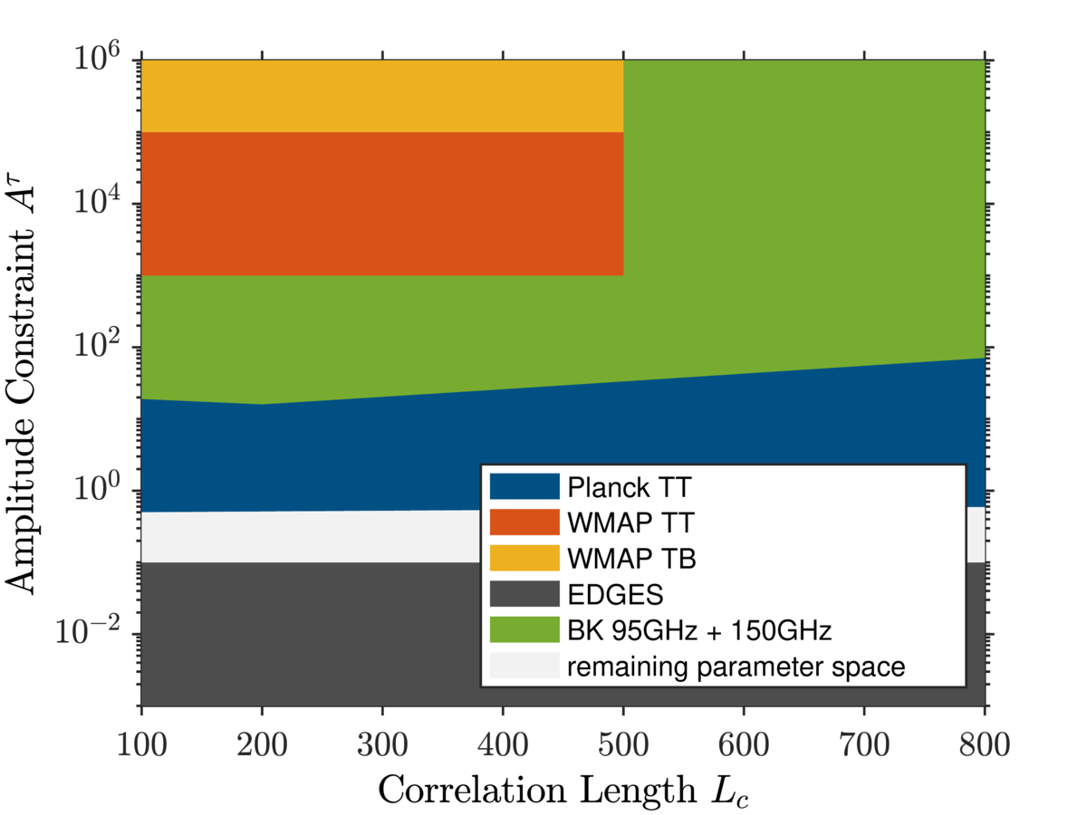
| Constraints on reionization |  |
Figure 6: Constraints on the amplitude \(A^\tau (L_c)\) of Equation (6) obtained from this work (green) and in the previous work (Gluscevic et al. 2013; Namikawa 2018). The colored regions are excluded. | PDF / PNG |
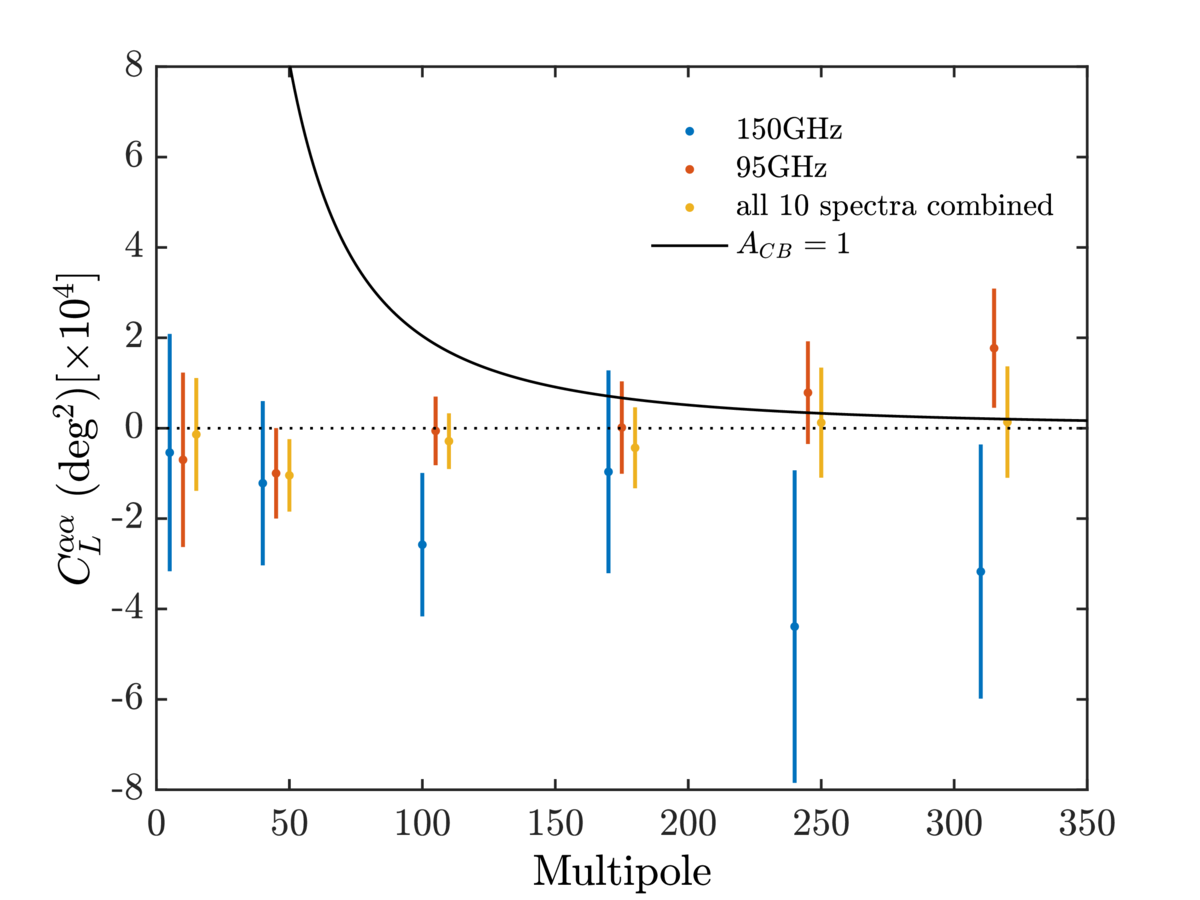
| Cosmic birefringence power spectrum | 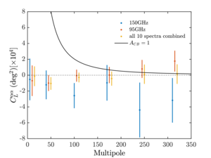 |
Figure 7: Cosmic birefringence power spectra \(\hat{C}_L^{\alpha\alpha}\) for 95 GHz only, 150 GHz only, and all 10 spectra combined. The black line is the fiducial spectra from Equation (43) with \(A_{CB}\) = 1. Compared to Figures 3 and 5, one additional bin of \(L \in [1,20)\) is separated out from the \(L \in [1,70)\) bin, since the lowest multipoles are important for constraining \(A_{CB}\). | PDF / PNG |
| Comparison of constraints on primordial magnetic fields | 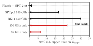 |
Figure 8: Comparing the constraint on the strength of PMFs smoothed over 1 Mpc, \(B_\mathrm{1Mpc}\), of this work with constraints from SPTpol anisotropic birefringence reconstruction (Bianchini et al. 2020) and Planck and SPTpol CMB power spectra (Zucca et al. 2017). | PDF / PNG |
| Distributions of jackknife PTE values | 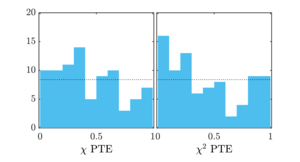 |
Figure 9: Distributions of the 84 \(\chi / \chi^2\) PTE values from 14 jackknives and three distortion fields of two real data frequency maps. | PDF / PNG |
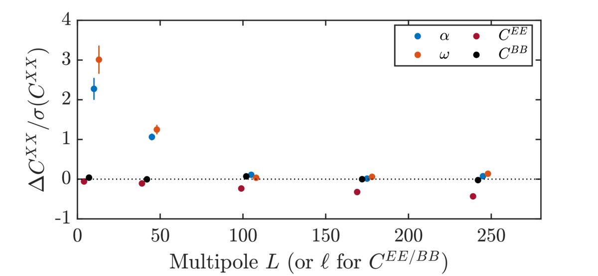
| Shifts in spectra from random 10° detector polarization angle scatter | 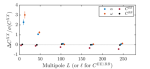 |
Figure 10: Mean shift in \(\alpha\), \(\omega\), \(EE\), and \(BB\) spectra in simulations with a 10° random detector polarization angle scatter divided by the standard deviation of the nonrotated simulations. Here \(\alpha\) and \(\omega\) pick up a strong signal at low L, while \(C_\ell^{EE}\) is suppressed at higher \(\ell\) because the random per-detector polarization rotations average out near the center of the map and reduce the overall amplitude. | PDF / PNG |
| Shifts in spectra from 10% differential gain fluctuations | 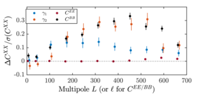 |
Figure 11: Mean shift in \(\gamma_1\), \(\gamma_2\), \(EE\), and \(BB\) spectra in simulations with a 10% Gaussian fluctuation of differential gain that varies from detector pair to detector pair and hour to hour divided by the standard deviation of the nonfluctuated simulations. | PDF / PNG |
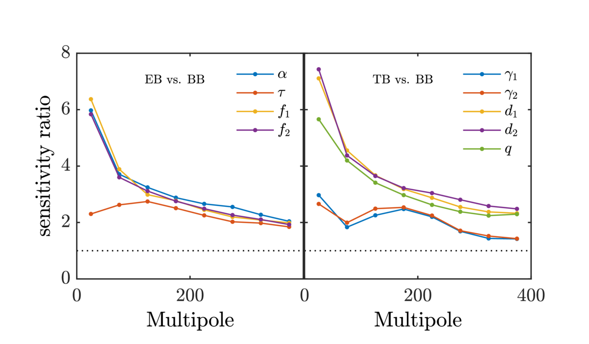
| Sensitivity ratio for quadratic estimators compared to \(BB\) spectrum | 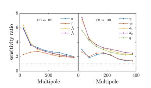 |
Figure 12: Sensitivity ratio as defined in Equation (58). A sensitivity ratio \(\sigma (A_D^{EB}) / \sigma (A_D^{BB})\) above 1 means that the quadratic estimator is more sensitive than the \(BB\) spectrum at detecting the distortion field at that angular scale. The left panel shows the sensitivity ratio for the fields involving only the polarization, while the right panel shows the fields involving \(T\). | PDF / PNG |
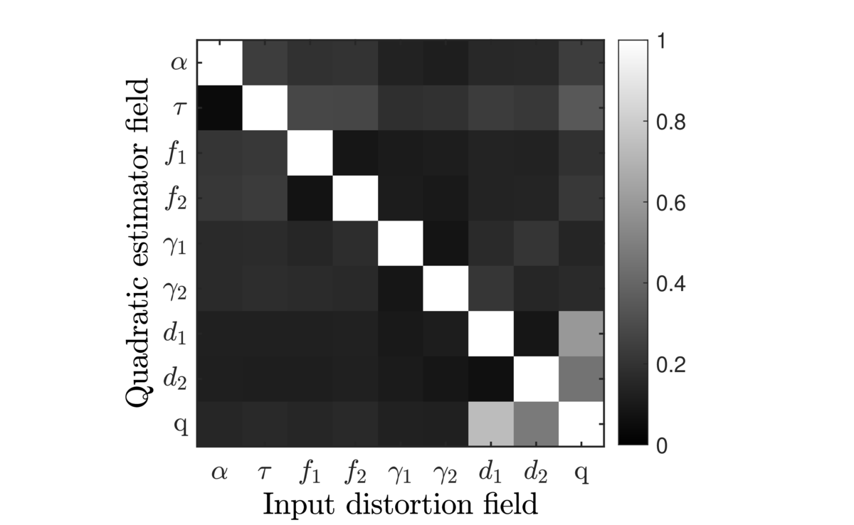
| Correlation matrix for quadratic estimators |  |
Figure 13: Correlation matrix of the sensitivity ratio as defined in Equation (58) for all combinations of input distortion and quadratic estimators. The results plotted use distortion input from \(L\) = 1 to 50. The horizontal axis shows the input distortion field injected in the simulations, and the vertical axis shows the quadratic estimators used to detect the signal. We see that \(q\) and \(d_1 / d_2\) have the strongest correlations, but in general, all of the distortion signals are best measured with their own estimators. | PDF / PNG |
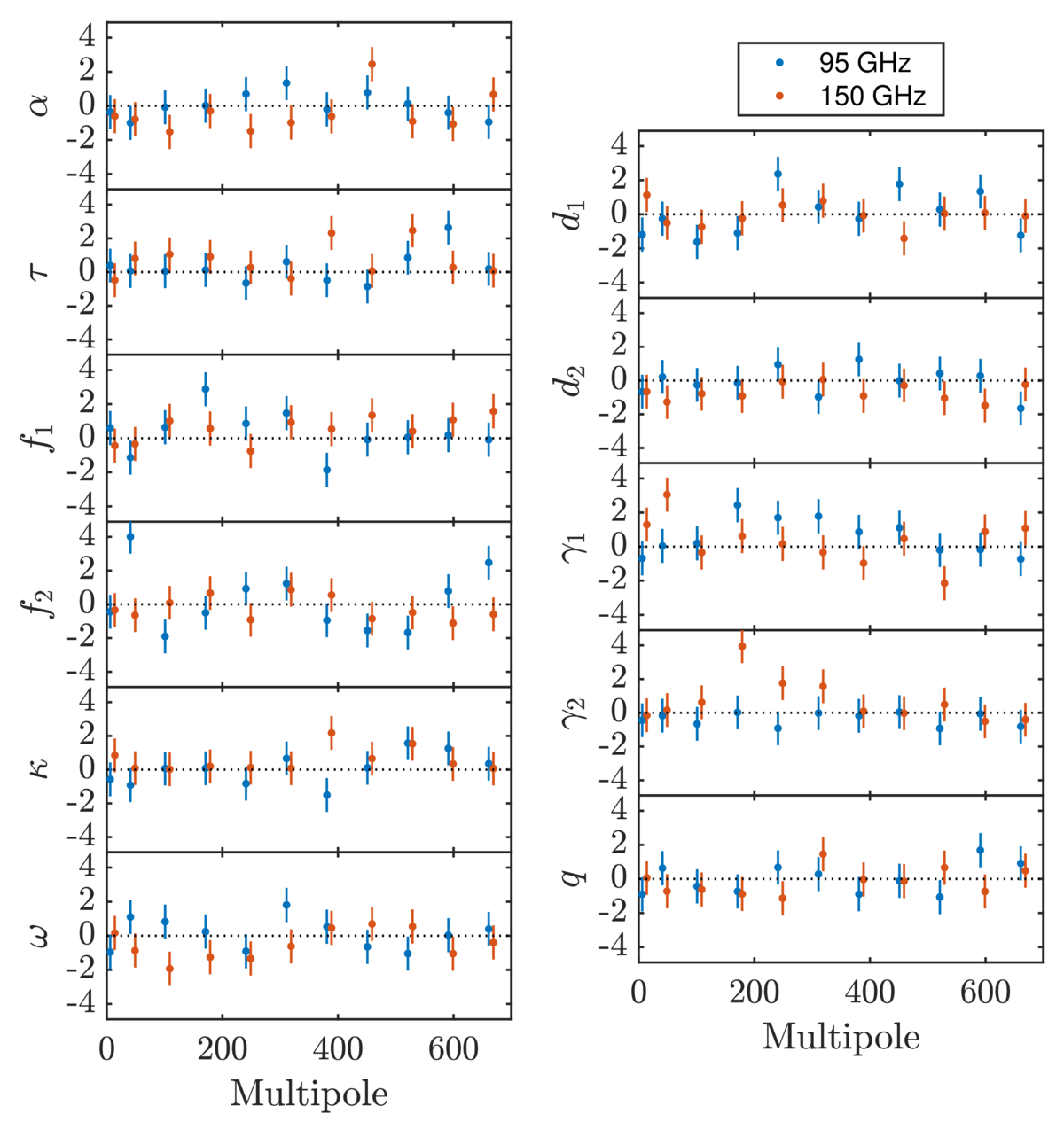
| Fractional deviations for real data distortion field bandpowers | 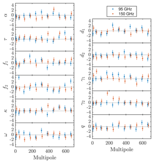 |
Figure 14: Fractional deviations of the 11 real data distortion field bandpowers \((\hat{C}_L^{DD} - \bar{C}_L^{DD}) / \sigma(\hat{C}_L^{DD})\). The plots on the left are reconstructed with the \(EB\) quadratic estimators, while the ones on the right are reconstructed with the \(TB\) estimators and have the point-source mask applied. The corresponding \(\chi\) and \(\chi^2\) PTEs are listed in Table 6. | PDF / PNG |
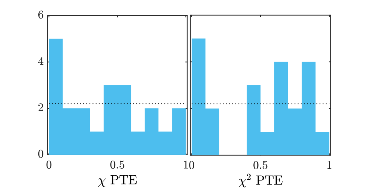
| PTE distributions for distortion systematic tests |  |
Figure 15: Distributions of the distortion systematics test \(\chi\) and \(\chi^2\) PTEs in Table 6. | PDF / PNG |
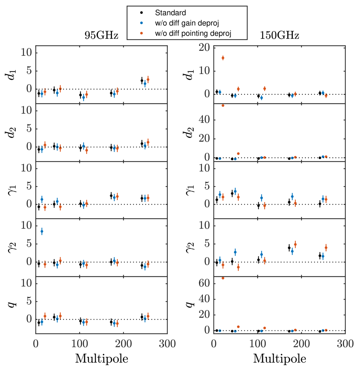
| Fractional deviations for real data distortion field bandpowers with or without deprojection | 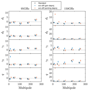 |
Figure 16: Fractional deviations of the 11 real data distortion field bandpowers \((\hat{C}_L^{DD} - \bar{C}_L^{DD}) / \sigma(\hat{C}_L^{DD})\) with and without the differential gain and pointing deprojections. Here 95 GHz fails the \(\gamma_2\) systematics test without differential gain deprojection, and 150 GHz fails the \(d_1\), \(d_2\), and \(q\) systematics tests without differential pointing deprojection. | PDF / PNG |
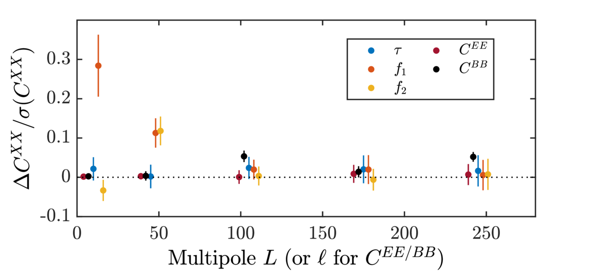
| Distortion field \(EE\) and \(BB\) difference spectra from systematics simulations |
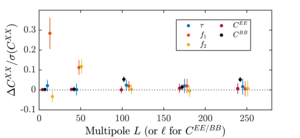 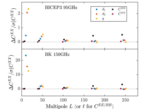
|
Figure 17: Relevant distortion field \(EE\) and \(BB\) difference spectra over the error bar \(\Delta C^{XX} / \sigma(C^{XX})\) from the different systematics simulations. Panels (a) and (c) are identical to Figures 10 and 11 of Section 6.1. (a) 10% random polarization angle rotation (b) 20% random pair averaged gain fluctuation (c) 10% hour to hour differential gain fluctuation (d) Dipole \(T\) to \(P\) leakage from beam map simulations with differential pointing deprojection turned off. |
PDFa / PNGa PDFb / PNGb PDFc / PNGc PDFd / PNGd |
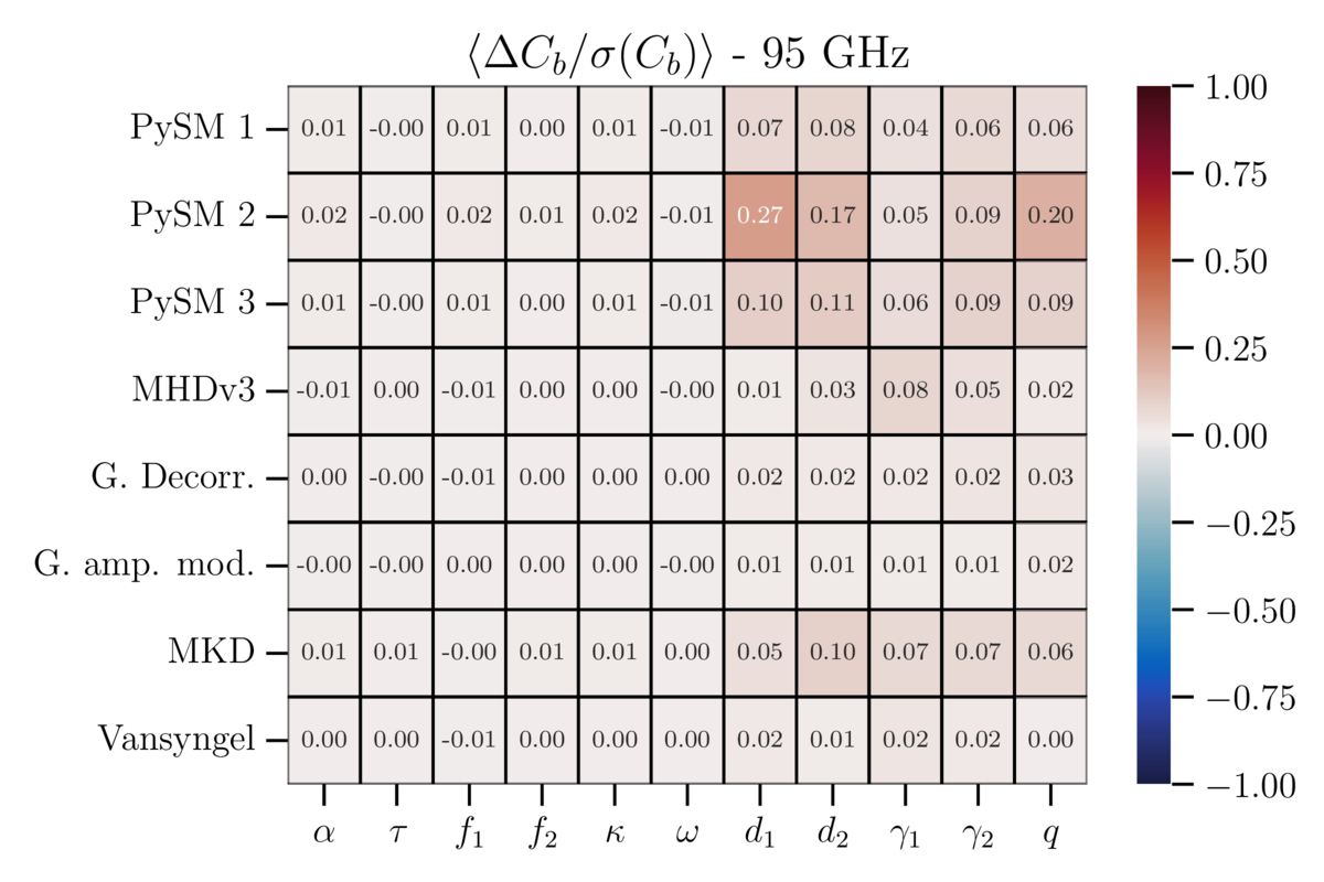
| Mean bandpower deviation for distortion fields | 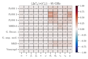 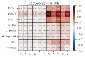 |
Figure 18: Mean bandpower deviation \(\left\langle \Delta C_b / \sigma(C_b) \right\rangle\) averaged over all bins for each of the 11 distortion fields. The choice of bins is the same as in Figures 14 and 16. | PDF1 / PNG1 PDF2 / PNG2 |
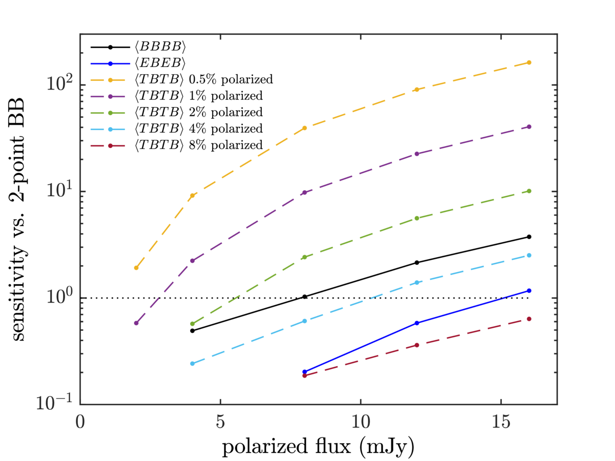
| Signal-to-noise ratio for detecting point sources with four-point estimators |  |
Figure 19: Signal-to-noise ratio for detecting the point sources of the different four-point estimators compared to two-point \(C_\ell^{BB}\) power in the BK18 95 GHz simulations. A sensitivity ratio larger than 1 on the y-axis means that the fourpoint estimator is more sensitive than the \(BB\) power spectrum at detecting that population (polarized flux and fraction) of point sources. Here \(\left\langle EEEE \right\rangle\) has too low a sensitivity to be probed by our simulations and is therefore not shown. | PDF / PNG |
History
- 2023-05-26: Posted BK-XVII: Line of Sight Distortion Analysis: Estimates of Gravitational Lensing, Anisotropic Cosmic Birefringence, Patchy Reionization, and Systematic Errors figures.