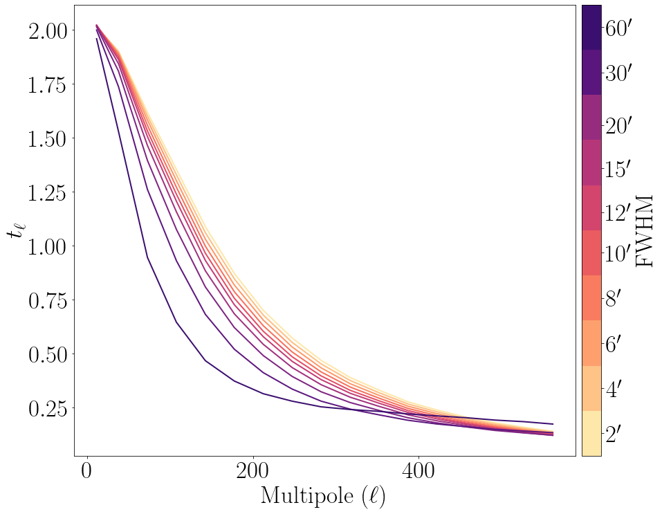
| RHT transfer function |
 |
Figure 1: The RHT algorithm multipole-dependent unitless transfer function defined in Equation 1 for different Gaussian smoothing FWHM values, computed on the Planck 70% sky fraction Galactic plane mask.
|
PDF / PNG |
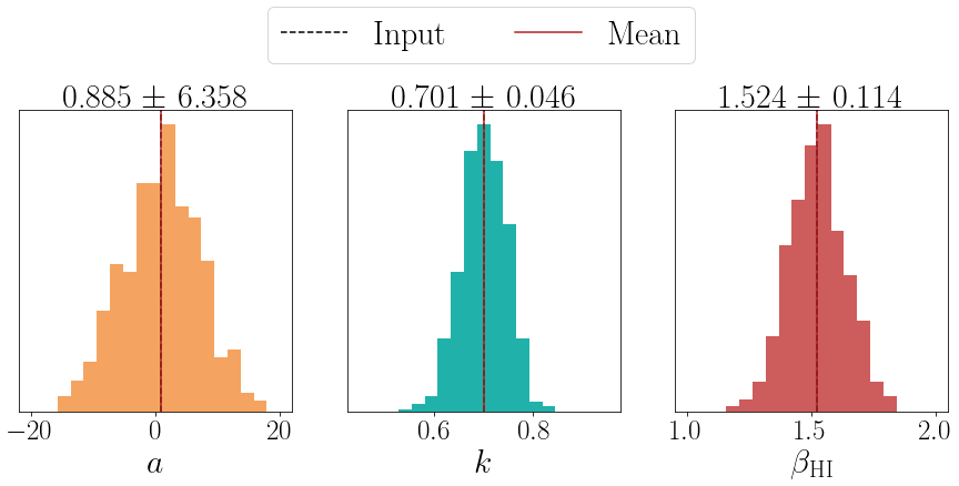
| Best-fit values from simulations |
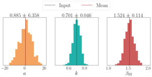 |
Figure 2: Distributions of the best-fit values using E and B modes for 499 realizations of lensed-ΛCDM, noise, and Gaussian dust, added to the HI morphology template with fixed input values a=0.9, k=0.7, and βHI=1.52 that match the fit from real data. The parameters a and βHI are unitless, and k has units μKCMB / K km s-1. These known input values are plotted as dashed black vertical lines. The means of the distributions of the best-fit values are plotted as solid red vertical lines. The mean and standard deviation of each of the distributions are quoted above.
|
PDF / PNG |
| Correlation of integrated HI template with individual velocity channels |
 |
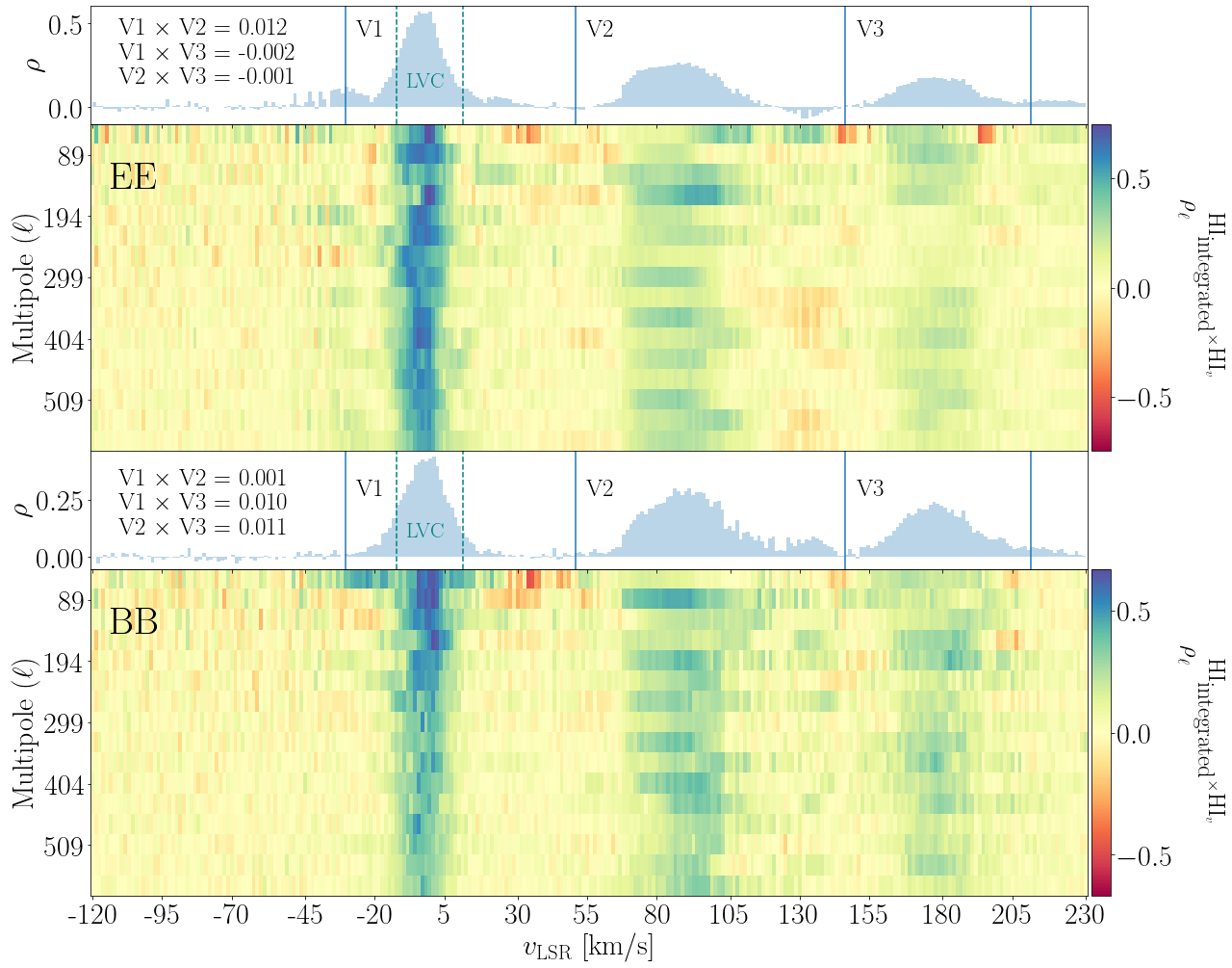
Figure 3: EE (top) and BB (bottom) correlation ratio of the integrated HI morphology template with individual HI morphology templates for the HI4PI velocity channels across multipoles 37 < ℓ < 579. The 1D plots on top show the broadband correlation ratio calculated over one multipole bin spanning the entire multipole range. Is is separated into 3 velocity regions, V1, V2, and V3. The LVC boundaries as defined in Panopoulou & Lenz (2020) are indicated with dashed vertical lines. The broadband correlation ratio between the different pair combinations of the 3 velocity components is printed on the left of each histogram.
|
PDF / PNG |
| Integrated HI intensity maps |
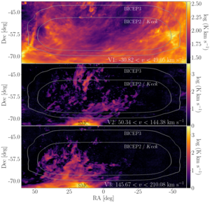 |
Figure 4: Integrated HI intensity maps over the 3 different velocity components defined in Figure 3 in the BICEP/Keck region. The velocity boundaries for each component are printed on the bottom right of each map. The emission in V1 is dominated by the Milky Way, whereas the emission in V2 and V3 is dominated by Magellenic Stream I (Westmeier 2018). The outlines of the BICEP3 and the BICEP2 and Keck Array observing fields are also plotted. The Small Magellenic Cloud (SMC) is indicated.
|
PDF / PNG |
| Polarized intensity maps using RHT parameters with high vs low B-mode correlation |
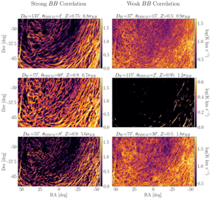 |
Figure 5: Polarized intensity maps of V1 in the BICEP/Keck region using RHT parameters that correlate > 5σ (left) and < 5σ (right) in B modes with BICEP/Keck and Planck data. Only the statistical significance in B modes is quoted in the title of each of the maps, because all of the RHT parameters we tried correlate well (> 5σ) in E modes. From top to bottom, the maps on the left have a 15.2σEE, 12.6σEE, and 14.9σEE detection significances, and the maps on the right have 6.3σEE, 8.6σEE, and 8.2σEE detection significances.
|
PDF / PNG |
| Velocity distribution of the HI structure |
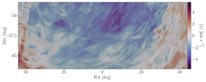 |
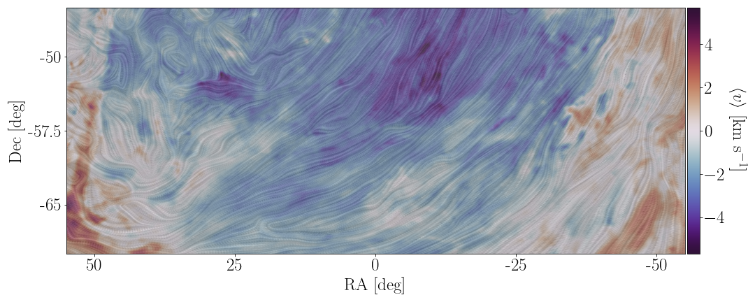
Figure 6: Map of the first moment of the velocity distribution of the HI structure in the BICEP/Keck region for -12 km s-1 < vlsr < 10 km s-1, the velocity range most correlated with the polarized dust emission. The texture is a line integral convolution of the magnetic field orientation as inferred by the HI filaments.
|
PDF / PNG |
| BB cross spectra with HI morphology template |
 |
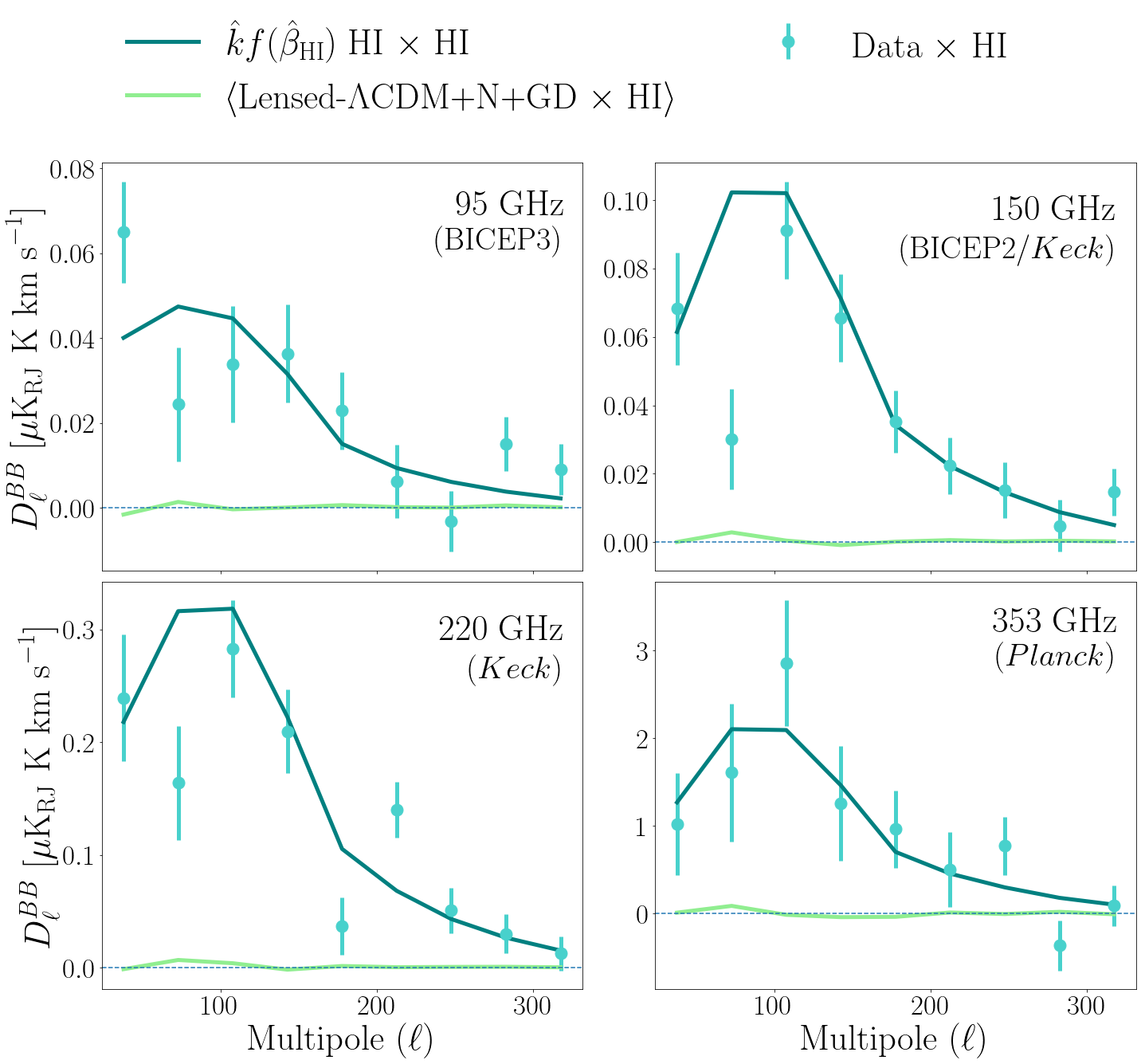
Figure 7: The best-fit BB observables used in the Δχ2 statistic defined in Section 3.6.2 for the 95, 150, and 220 GHz bands of BICEP/Keck and the 353 GHz band of Planck. A modified blackbody frequency scaling, covariance matrix conditioning, and a transfer function for the HI morphology template with the RHT parameters from Equation 13 are used for the fit here. The cross spectrum between the real data and the HI morphology template (light blue), the best-fit cross spectrum between the HI morphology template and the modified HI-correlated component of the simulation (dark blue), and the mean of the cross spectra between the HI morphology template and the lensed-ΛCDM, noise, and Gaussian-dust components of the simulation (light green) are plotted.
|
PDF / PNG |
| Posteriors of k and βHI |
 |
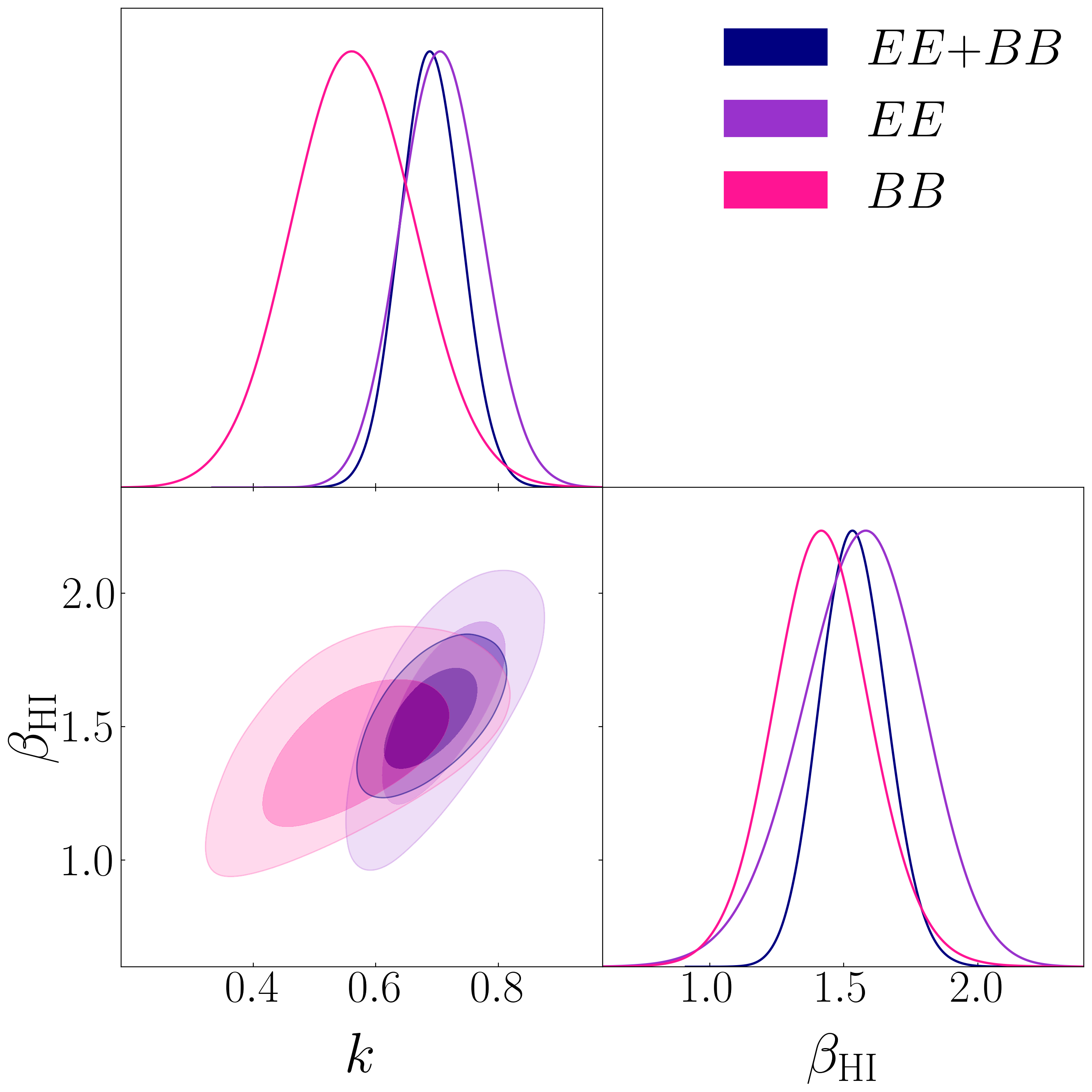
Figure 8: Posteriors of k and βHI fit using the Metropolis-Hastings algorithm on uniform priors and the χ2 likelihood of the cross spectra of the real data with the HI morphology template. The parameter a is marginalized over. The E modes only (purple), B modes only (pink), and simultaneous E and B modes (navy) posteriors are shown. The units for k are μKCMB / K km s-1 and βHI is unitless.
|
PDF / PNG |
| Comparisons of β posteriors for total vs filamentary dust components |
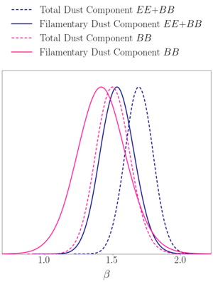 |
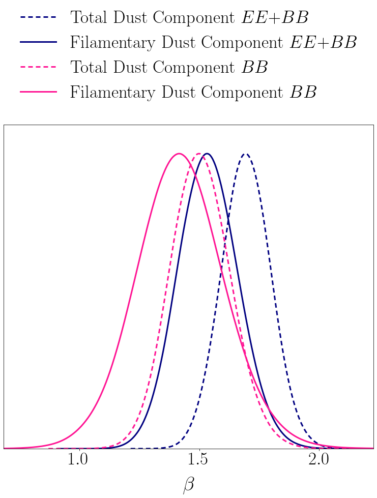
Figure 9: Comparison of the posteriors for βHI through a χ2 likelihood using cross correlations with the HI morphology template (solid) to the ones of βd using the Hamimeche and Lewis (HL) likelihood with a multicomponent model and no HI morphology template (dashed). We show the posteriors using B modes only (pink), and B and E modes (blue). The solid posteriors are the same as in Figure 8 plotted with the same colors. The B-mode-only total dust component posterior is identical to the posterior shown in black in Figure 4 of BK18.
|
PDF / PNG |
| Comparison of β posteriors for different data selections |
 |
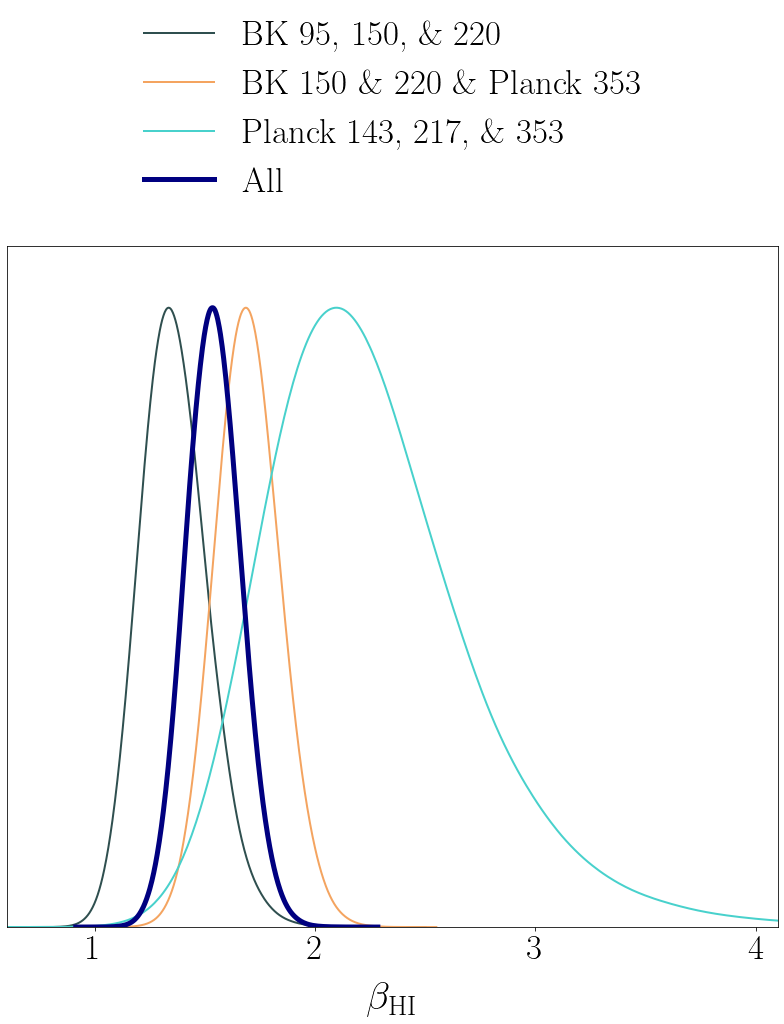
Figure 10: Comparison of the posteriors for βHI we get through a χ2 likelihood using E- and B-mode cross correlations with the HI morphology template for different selections of frequency bands and for BICEP/Keck only and Planck only variations. The thick navy posterior labeled “All” is the same as the navy posterior in Figures 8 and 9.
|
PDF / PNG |
| Correlation ratios between V1 and BICEP/Keck or Planck data |
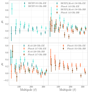 |
Figure 11: EE (cross) and BB (circle) unitless correlation ratios as a function of multipole moment. The correlation ratios between V1 and Planck data with 1σ variations are shown in red and brown to compare them to the correlation ratios V1 and BICEP/Keck data, which are shown in teal and turquoise. The errors are derived from spurious correlations between V1 and lensed-ΛCDM, Gaussian dust, and noise. Data points for similar frequencies between BICEP/Keck and Planck are plotted on the same panels for comparison.
|
PDF / PNG |
| Cross spectra between V1 and BICEP/Keck or Planck data |
 |
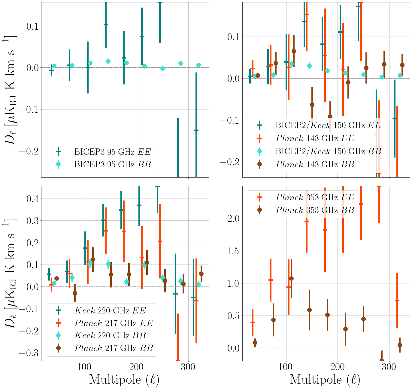
Figure 12: EE (cross) and BB (circle) cross spectra as a function of multipole moment. The cross spectra between V1 and Planck data with 1σ variations are shown in red and brown to compare them to the cross spectra between V1 and BICEP/Keck data, which are shown in teal and turquoise. The errors are derived from spurious correlations between V1 and lensed-ΛCDM, Gaussian dust, and noise. Data points for similar frequencies between BICEP/Keck and Planck are plotted on the same panels for comparison.
|
PDF / PNG |