-
BK-XIX: Extremely Thin Composite Polymer Vacuum Windows for BICEP and Other High Throughput Millimeter Wave Telescopes
The BICEP/Keck Collaboration, ApJ 1000, 238, 2026
| Figures | Download Bundle | ||
|---|---|---|---|
| Optical loading and relative NET from windows | 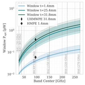  |
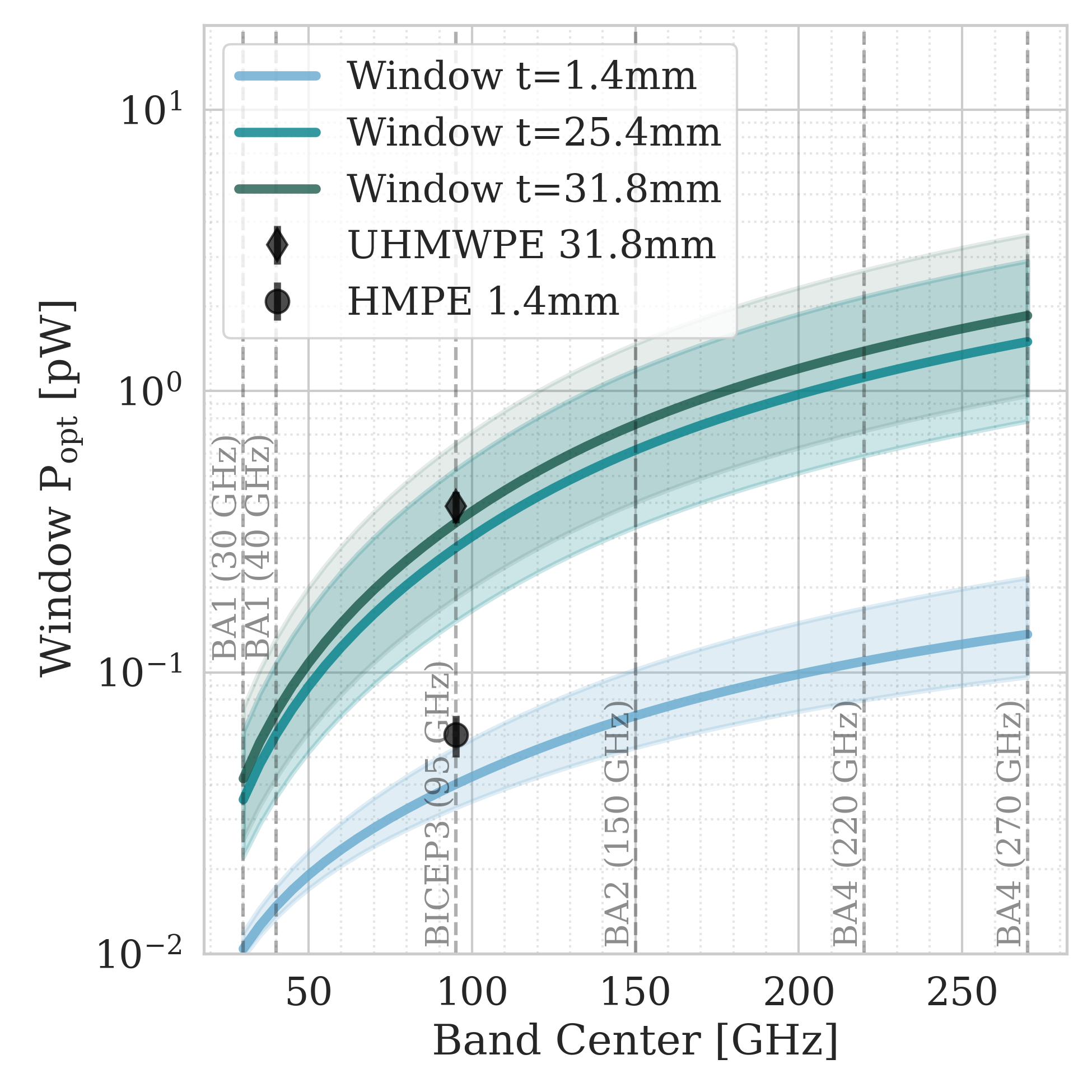
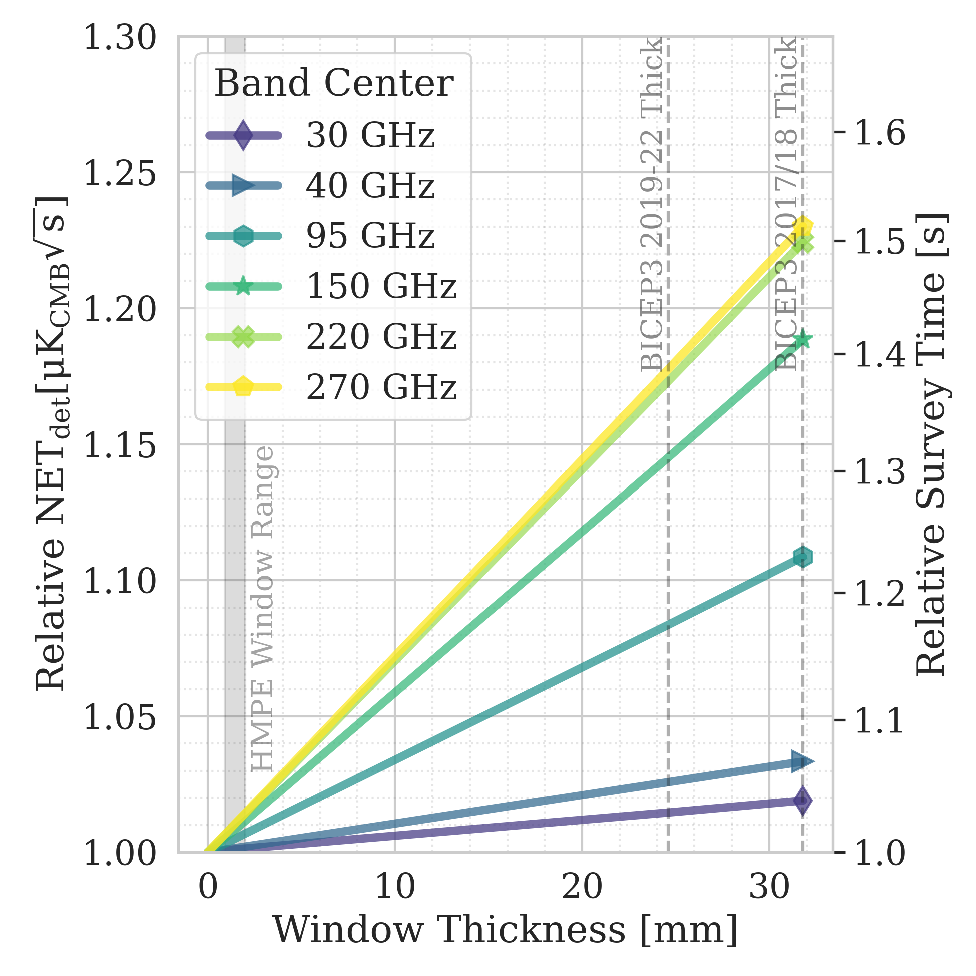
Figure 1: [a] Modeled optical loading from a window with thicknesses of 1.4 mm, 25.4 mm, and 31.8 mm, at band centers from 30 to 270 GHz (fractional bandwidth of 0.25) through a BICEP-style instrument. Black points are measured optical loading on BICEP3 from a 31.8 mm (1.25″) UHMWPE spare window and the 1.4 mm laminate window deployed on BICEP3 for the 2023 season. Shaded bands are uncertainty on the loss properties of the window, with tan δ between \(0.6\times10^{-4}\) to \(2.4\times10^{-4}\). [b] Modeled relative noise equivalent temperature per detector (NETdet) and the relative survey time increase compared to an instrument without a window, for each of the BICEP Array observing band center frequencies. | PNGa PNGb |
| BICEP3 cutaway detail | 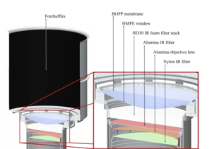 |
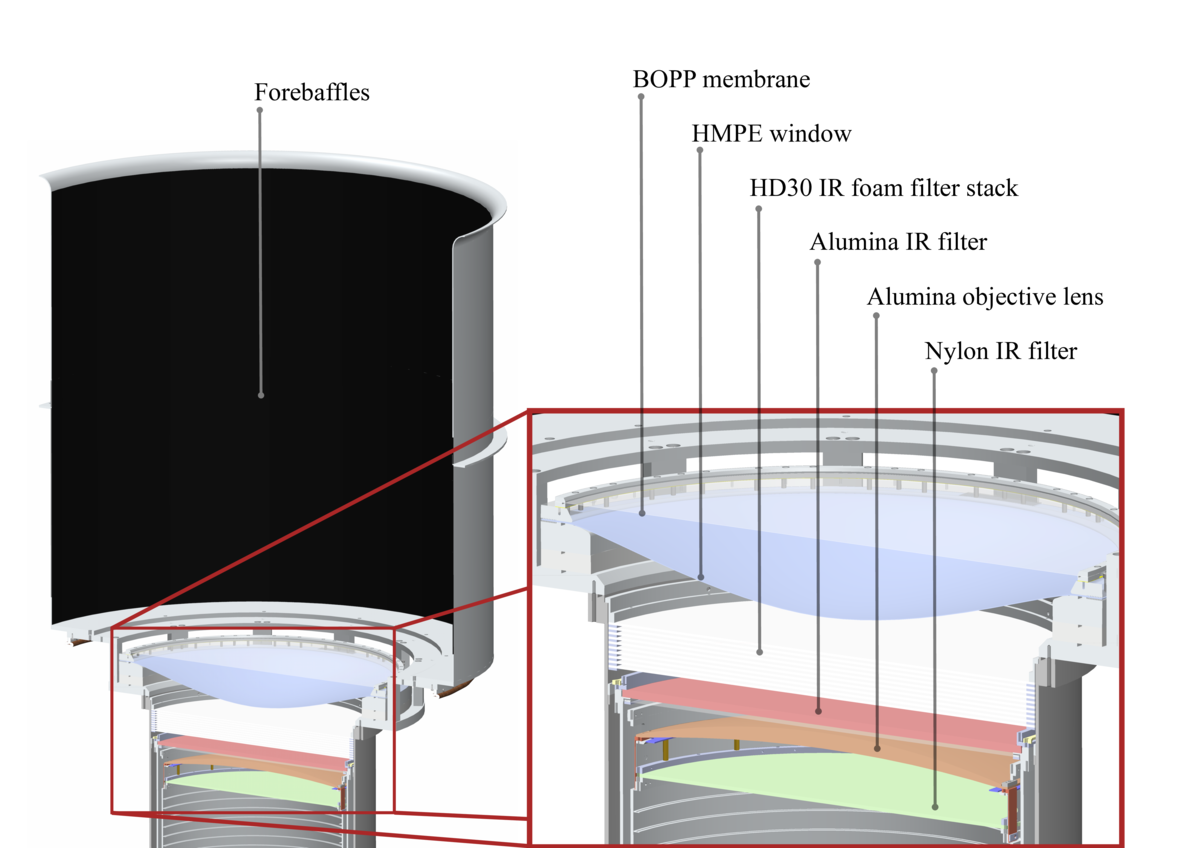
Figure 2: A cutaway of the top portion of the BICEP3 cryostat. Displayed from top to bottom are the forebaffles, BOPP membrane (to contain warm circulated air above the window), thin HMPE window, HD30 IR foam filter stack, alumina IR filter, alumina objective lens, and first nylon IR filter. The rest of the cryostat is described in Figure 6 of BK-XV. The thin HMPE window in this model is deflected 75 mm, with the foam filters remaining 45 mm away from the window. | PDF / PNG |
| Laminated window samples | 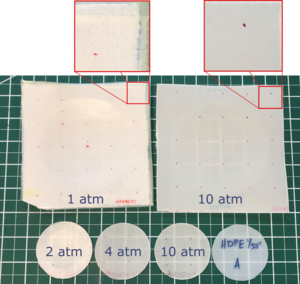 |
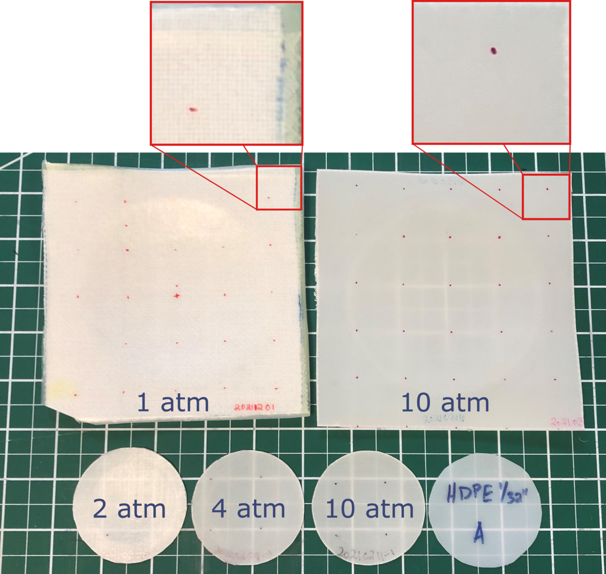
Figure 3: Photo of several small scale laminated window samples, labeled with the pressure at which they were laminated in atmospheres (atm). The top two samples were used in the permeation tests in Figure 7; the recipes are identical apart from the difference in lamination pressure. Note that the weave of the HMPE fibers remains visible in the 1 atm laminated, whereas the 10 atm laminate appears more homogeneous. Below these is a row of three smaller HMPE laminate samples and a solid extruded HDPE sheet having the same thickness. The highest pressure (10 atm) laminate (top right and bottom second to the right) is visually most similar to the solid HDPE sample. Note that the grid pattern on the mat below the samples laminated at lower pressure is blurred by light scattering associated with the incomplete filling of the HMPE weave with LDPE. | PDF / PNG |
| Tensile strength tests | 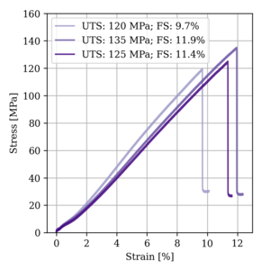 |
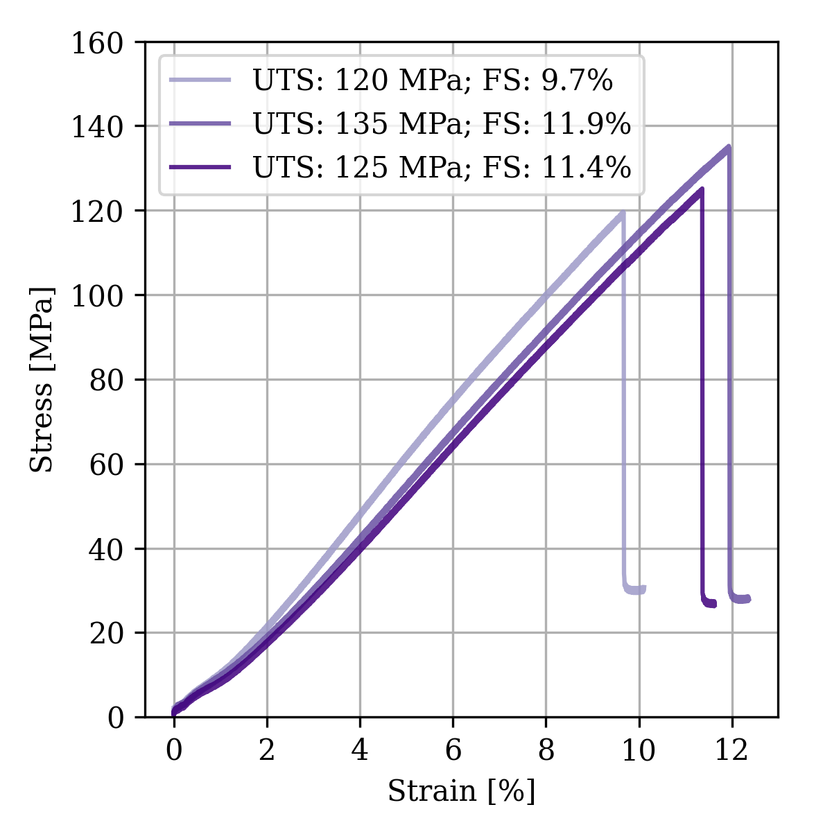
Figure 4: Tensile strength tests of three samples from a high pressure (10 atm, 135°C) HMPE laminate. The stress is calculated by dividing the measured force by the initial cross sectional area of the sample, while the strain is the percent change in elongation. The ultimate tensile strength (UTS) and the failure strain (FS) for each sample are reported in the legend, and summarized and compared to other polyethylenes in Table 1. | PNG |
| Hydrostatic test | 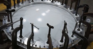 |
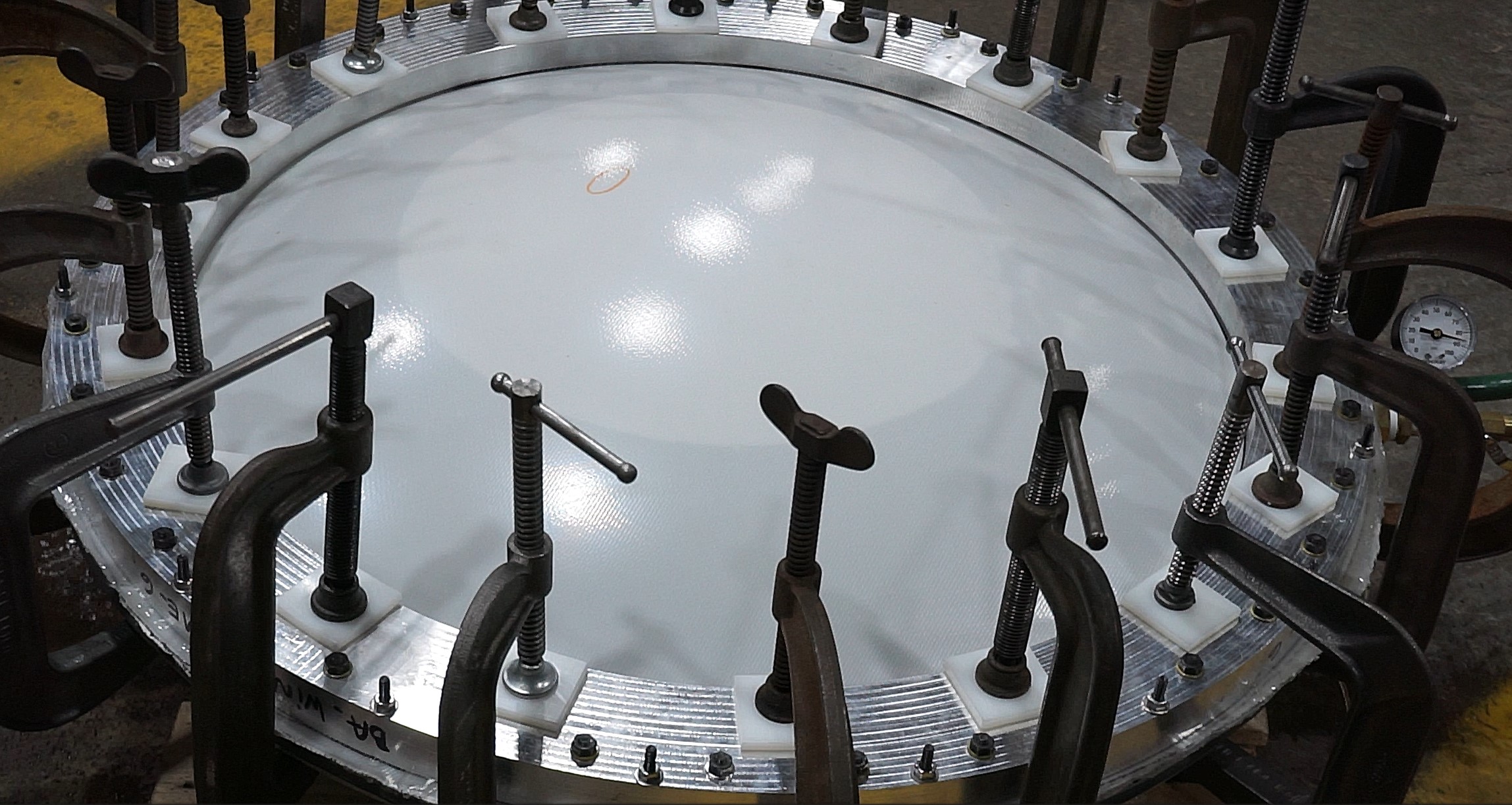
Figure 5: Photo of the window at the highest pressure achieved during the hydrostatic test. The pressure gauge (center right) reads approximately 85 psi (5.7 atm), and there is water leaking out around the gasket seal on the left hand side. | JPG |
| Window center deflections and strain | 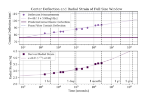 |
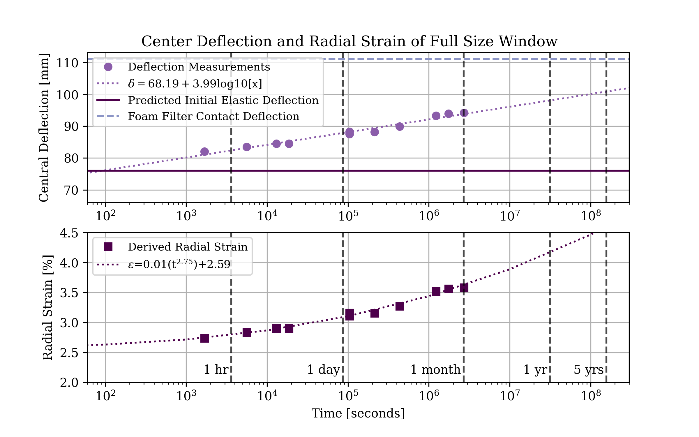
Figure 6: [Top] Measured center deflections of a window on a BICEP Array scale cryostat. The purple solid line denotes the predicted elastic deflection from the plate equation Eq. 1 using a radius of 400 mm. The light purple dashed line denotes the deflection at which contact would be made with the foam infrared filters behind the window. [Bottom] Estimated radial strain using Eq. 3 and the measured deflections. | PNG |
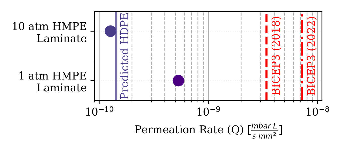
| Gas permeation rate | 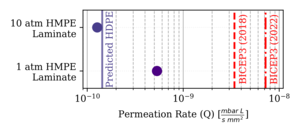 |
Figure 7: Measured permeation rates of small samples (circles) compared to the predicted rate with equivalently thick bulk HDPE from literature (solid line) and two limits on permeation from the unacceptable maximum rate of gas accumulation in two years; a marginally acceptable rate from BICEP3 in 2018 (dashed line) and an unacceptably high rate from BICEP3 in 2022 (dot-dashed line). The predicted HDPE value is calculated with Eq. 5, the permeation constant from Nguyen-Tuong (1993), and the laminate sample thickness. The two upper limit rates are determined through final warm pressure measurements (reported in Table 2) assuming that all the gas entered through the window over the time the BICEP3 cryostat was under vacuum. Both laminates are shown in Fig. 3. The high pressure (10 atm) laminate has a permeation rate closest to the bulk HDPE permeation rate. | PNG |
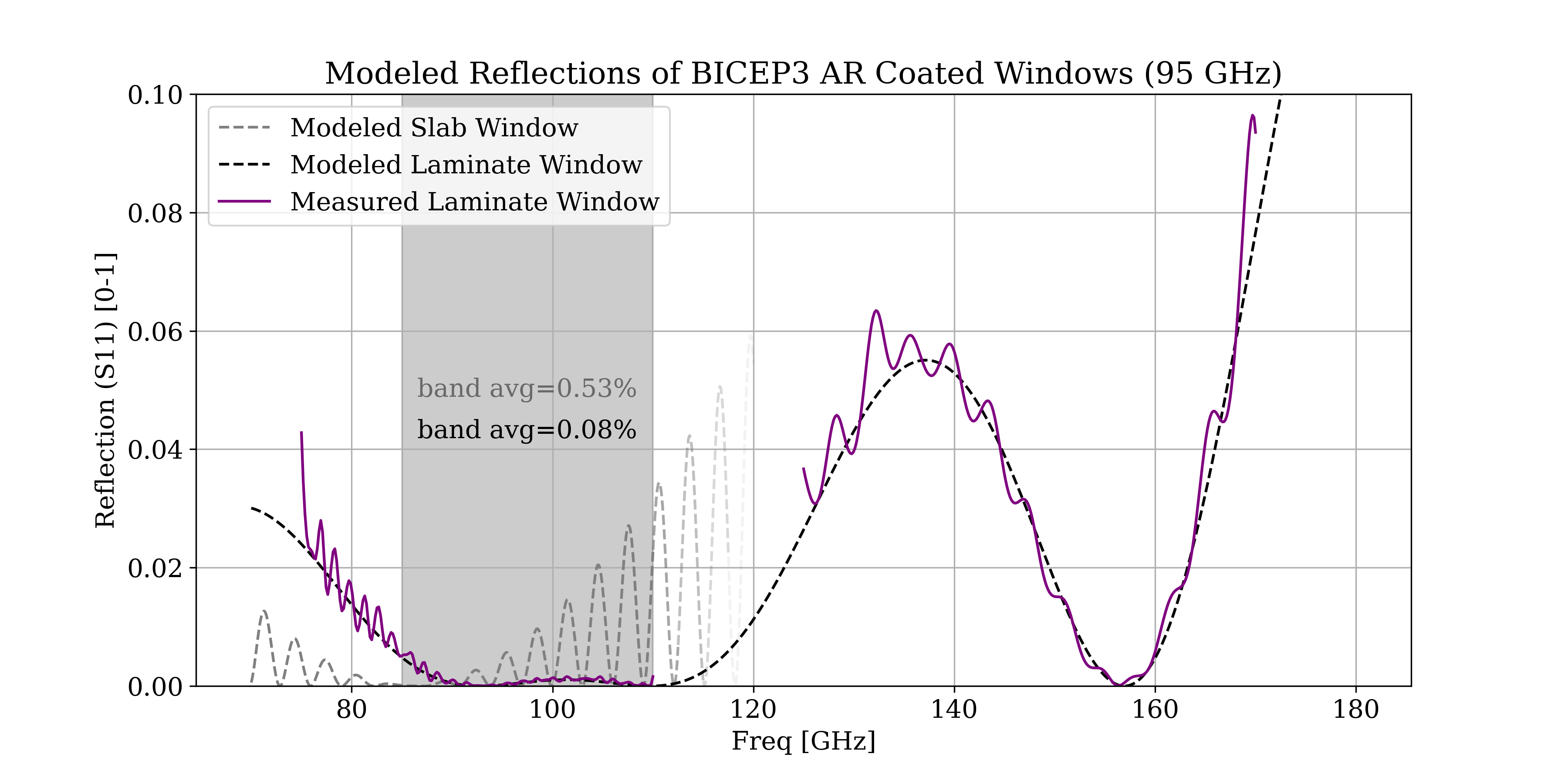
| AR coat model and measurements | 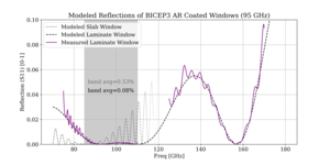 |
Figure 8: Measured VNA S11 reflections of the BICEP3 thin window (solid purple lines, both in-band WR 10 and out of band WR 6.5), and modeled reflections of the laminate (dashed black line) and the slab window (dashed gray line). The average in-band reflection of the AR coated slab is estimated to be 0.53% while the average in-band reflection of the AR coated laminate is estimated to be 0.08%. The in-band and out-of-band measurements on the laminate window show excellent consistency with the modeled reflection. | PNG |
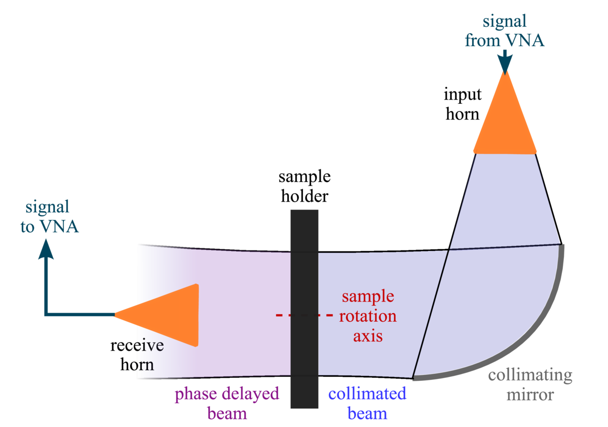
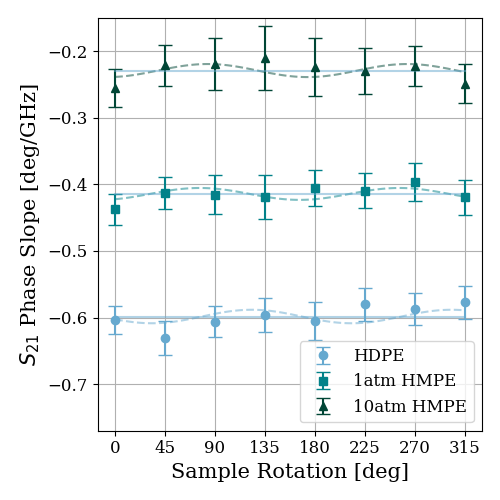
| Phase offset birefringence measurement | 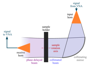 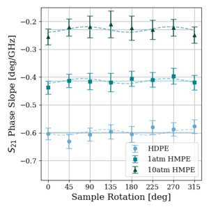 |
Figure 9: [a] Diagram of phase offset measurement (not to scale). Millimeter wave signal comes from the VNA and is coupled to free space through the input horn and collimated by the parabolic mirror. The collimated beam then interacts with the sample in the sample holder orthogonal to the propagation axis, where the phase will be delayed by the sample's electrical length. The receive only horn then couples the signal back into the VNA (S21 phase measurement). [b] Fit phase slopes for S21 phase offset measurements of 0.79 mm (1/32″) thick HDPE and the two HMPE laminates, one baked at 1 atm (0.68 mm thick) and the other baked at 10 atm (0.4 mm thick). If the materials are not birefringent then the phase slope should not vary significantly with sample rotation. If the materials exhibit uniaxial birefringence, we would expect the same phase slope on measurements 180 deg rotated from each other: we have fit both a flat line (solid lines) and a sin(2θ) wave (dashed lines) to the data to test the maximum amplitude of the possible phase offsets for each material. | PDFa / PNGa PNGb |
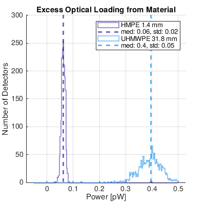
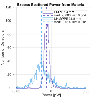
| Excess loading and scattered power from windows | 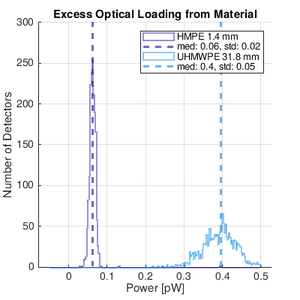 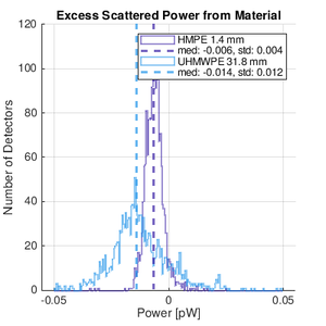 |
Figure 10: [a] Histograms of excess loading per detector from two different windows placed above BICEP3. [b] Histograms of scattered power to the forebaffle associated with placing the material in front of the BICEP3 receiver. Blue line is a spare UHMWPE 31.8 mm (1.25″) thick window for BICEP3; dashed line denotes the median excess load from the slab. Purple line is the replacement HMPE 1.4 mm thick window for BICEP3; dashed line is the median excess load from the laminate. | PNGa PNGb |
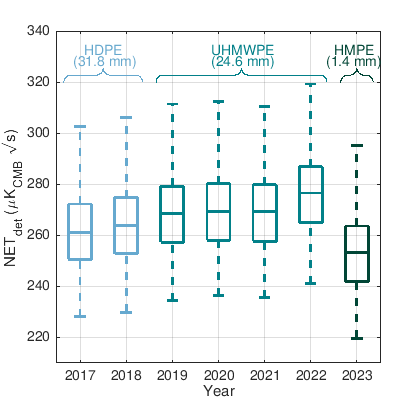
| BICEP3 NET vs year |  |
Figure 11: BICEP3 median white noise (NET) distribution over all detectors per year between 2017 and 2024. Per detector per scanset (roughly 50 minutes of time ordered data) NETs are calculated, then a median per detector over the entire year's scansets are shown, with 25th (q25), 50th, and 75th (q75) percentiles shown in the box, to demonstrate average noise of the receiver between years. Whiskers cover the remainder of the distribution, excluding outliers, defined by q25/75±(q75-q25). Color corresponds to the kind of window on the receiver: light blue is HDPE 31.8 mm (1.25″), blue is UHMWPE 24.6 mm (0.97″), and dark green is HMPE 1.4 mm. There is a significant change in noise between three observing seasons: 2018–2019, 2021–2022, and 2022–2023. | PNG |
| Modeled vs measured NET | 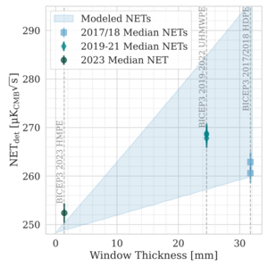 |
Figure 12: Median measured NETs (white noise) from Figure 11 as a function of the window thickness for that respective year. We exclude 2022 due to elevated optics temperatures. The blue shaded band of NET models show predicted BICEP3 NET values, varying the window loss tangent between \(0.6\times10^{-4}\) to \(2.4\times10^{-4}\). We have not yet concluded on the cause of the increase in the white noise measured between the thicker HDPE window (31.8 mm) in 2018 to the UHMWPE window (25.4 mm) in 2019: both a difference in material loss and a difference in scattering properties could explain this change. The HMPE window did definitively and significantly decrease the measured white noise compared to both thick slab windows. | PNG |
History
- 2026-07-15: Updated to match version published by ApJ.
- 2025-07-08: Posted BK-XIX: Extremely Thin Composite Polymer Vacuum Windows for BICEP and Other High Throughput Millimeter Wave Telescopes figures.