| Pipeline diagram |
 |
Figure 1: Flow diagram of the axion-oscillation analysis pipeline. The three main components are indicated on the left, and more detail is presented in the rest of the figure. The map-making step is similar to that of a standard CMB analysis, though the reobservation must now include a component that represents polarization oscillations (Secs. III B, III D and III G). The coadds are estimates of the time-averaged Stokes parameters \( \left\langle Q(\hat{n}) \right\rangle \) and \( \left\langle U(\hat{n}) \right\rangle \). The global rotation angle \(f(t) / 2\) is obtained through the correlation method of Sec. III E with some of the computational speed-ups of Sec. III G. The likelihood and Bayesian analysis are described in Sec. IV. The ensemble of simulations is used to construct a model distribution, which we can resample to form large numbers of Gaussian pseudo-simulations (Sec. IV A 1). The model distribution also implies a likelihood function (Sec. IV B) that is used to set Bayesian upper limits (Sec. IV C). At the same time, we estimate test statistics to check consistency with the background model (Sec. IV D) and to test for spurious systematic signals (Sec. V). Based on the results of the systematics checks, which we call “jackknife tests”, we unblind the real non-jackknife data (Sec. VI B).
|
PDF / PNG |
| Illustration of correlation method |
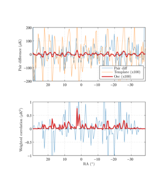 |
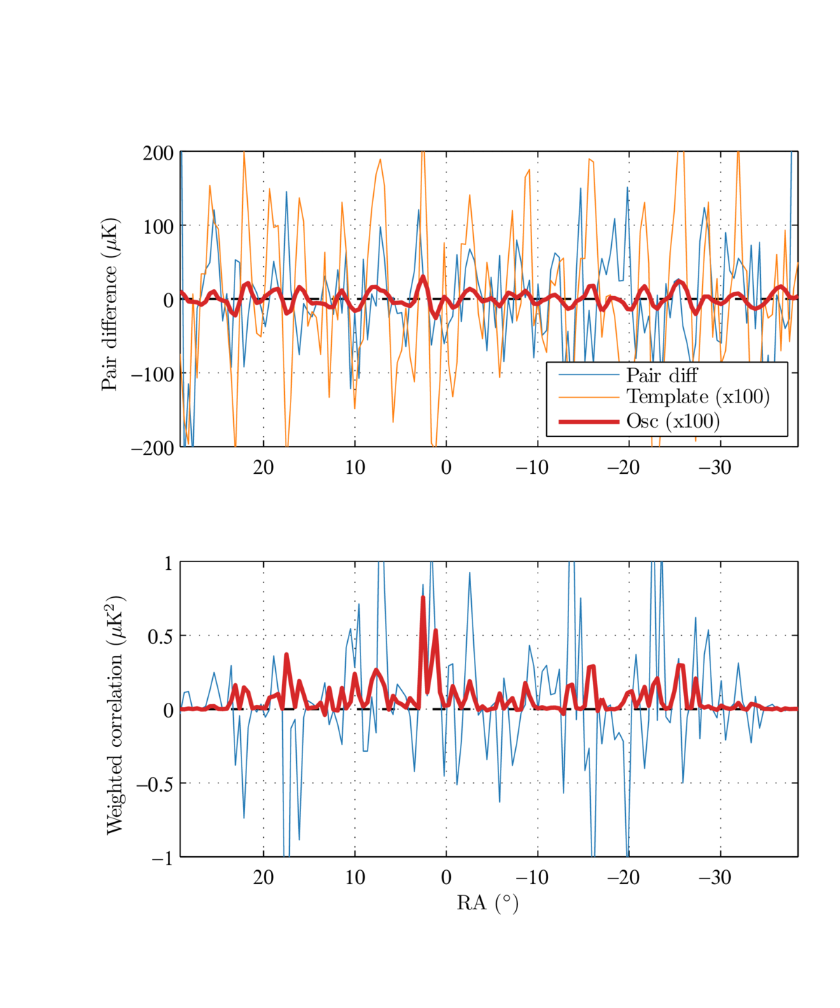
Figure 2: An illustration of the correlation method introduced in Sec. III E for a simulation of a single detector and a single observation. (Top) The pair difference \( \bar{D}_i ( \hat{\bf n}, \tau ) \) (blue) from a constant-elevation scan is plotted against right ascension (RA). The pair difference is dominated by atmospheric loading and fluctuates strongly. In this simulation, a global rotation of 3° has been imposed. The oscillating component \( \bar{D}_i^\mathrm{(osc)} ( \hat{\bf n}, \tau) \) (red) is hidden underneath the atmospheric fluctuations. The rotated map \( \bar{r}_i (\hat{\bf n}, \tau ) \) (orange) is used as a template to pick out global polarization rotations. (Bottom) The correlation \( \rho(\tau) \) (Eq. 20 summed over detector \(i\) only) between the template and the full pair difference (blue) has a large variance but mean zero. The correlation with the oscillating component (red) is biased positive.
|
PDF / PNG |
| Simulated time series |
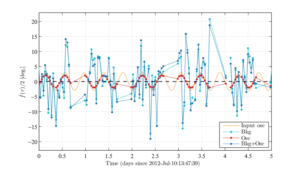 |
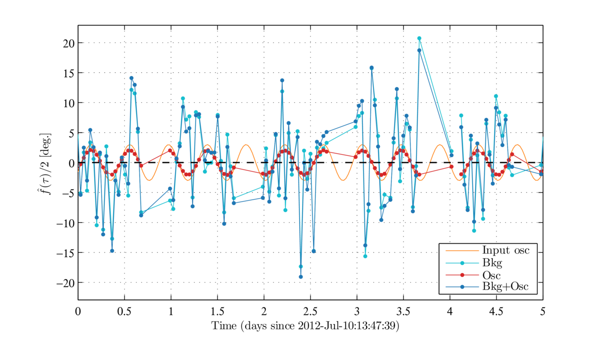
Figure 3: A simulated time series \( \hat{f}(\tau) \) (blue) with an input rotation amplitude \(A/2 = 3\)°, chosen to be relatively large in order to illustrate the effect more clearly. The background \( \hat{f}^\mathrm{(bkg)} (\tau) \) (cyan, defined explicitly in Eq. 51) dominates over the oscillating component \( \hat{f}^\mathrm{(osc)} (\tau) \) (red, Eq. 50). The template maps \( \bar{Q} (\hat{\bf n}) \) and \( \bar{U} (\hat{\bf n}) \) are constructed from standard BICEP simulations of only the 2012 observing season of the Keck Array, so the underlying true oscillation \( f(t) \) (orange) is not recovered at full strength but is instead suppressed by ∼30% as described in Sec. III F.
|
PDF / PNG |
| Test statistic for consistency with background model |
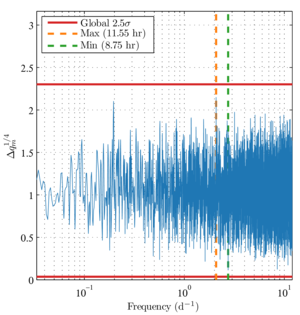 |
Figure 4: The test statistic \( \Delta q_m \) for consistency with the background model (Eq. 65) for real data from the 2012 observing season of the Keck Array. We plot \( \Delta q_m^{1/4} \) on the vertical axis in order to compress the distribution for visual purposes, and we plot frequency \( m / (2 \pi) \) in units of inverse days (\( \mathrm{d}^{-1} \)) on the horizontal axis. The maximum and minimum values are indicated in the legend with their corresponding oscillation periods. The levels for global \(2.5 \sigma\) fluctuations in both directions are indicated by horizontal red lines, i.e., there is a 1.2% probability in the background model that at least one value of \( \Delta q_m \) will lie outside the region bounded by the red lines.
|
PDF / PNG |
| Bayesian 95% confidence upper limits |
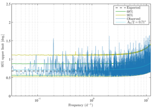 |
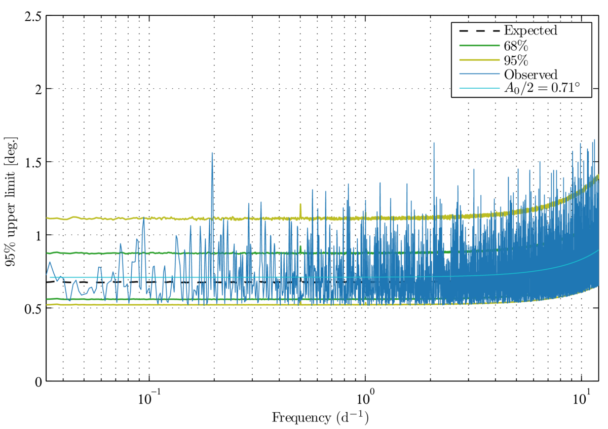
Figure 5: Bayesian 95%-confidence upper limits on rotation amplitude \(A/2\) (Sec. IV C). We also provide the median expectation (black dashed) from background-only simulations as well as \(1 \sigma\) (green) and \(2 \sigma\) (yellow) regions. These expectations represent local rather than global percentiles. With nearly \(10^4\) frequencies under consideration, we expect several values outside of the \(2 \sigma\) region. The question of background consistency is addressed by Fig. 4 and the test statistic \( \Delta \hat{q} \) (Eq. 66). The median limit for oscillation periods larger than 24 hr (frequency less than 1 \(\mathrm{d}^{-1}\)) is 0.68°. For shorter periods (larger frequencies), the limits are degraded due to binning observations in ∼1-hr scansets (Sec. III C). Additionally, we plot a smoothed approximation to our upper limits (Eq. 76) in cyan.
|
PDF / PNG |
| Exclusion plot |
 |
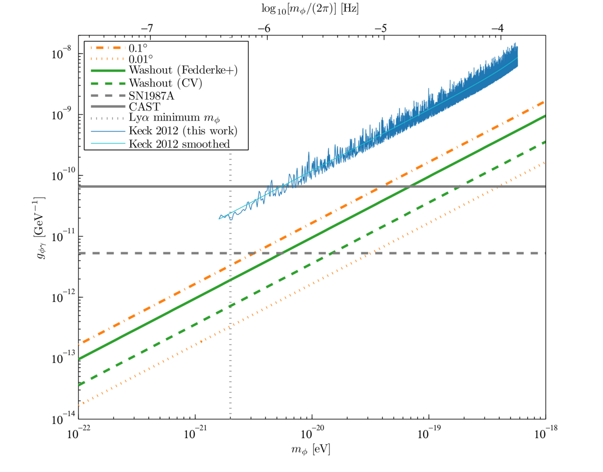
Figure 6: Excluded regions in the mass-coupling parameter space for axion-like dark matter (cf. Fig. 3 in [12]). All constraints push the allowed regions to larger masses and smaller coupling constants, i.e., toward the bottom right of the figure. If the dark matter is assumed to consist entirely of axion-like particles, i.e., if \( \kappa = 1 \), then our constraints (blue) are immediately implied by Eq. 78 and the results of Fig. 5. A smoothed approximation is shown in cyan (Eq. 79). The orange dot-dashed and dotted lines show the constraints that would be achieved if the rotation amplitude were constrained to 0.1° and 0.01°, respectively. The green solid line shows the constraint set by Fedderke et al. [12] by searching for the washout effect (Sec. I) in publicly available Planck power spectra. The dashed green line shows the cosmic-variance limit for the washout effect. The dashed grey horizontal line shows the limit from searching for a gamma-ray excess from SN1987A [23]. The solid grey horizontal line is the limit set by the CAST experiment [26]. The dotted grey vertical line is a constraint on the minimum axion mass from observations of small-scale structure in the Lyman-α forest [27], though we note that several similar bounds have also been set by other considerations of small-scale structure [28, 29].
|
PDF / PNG |