1. BICEP2 2014 Release Papers
-
BICEP2 2014 I: Detection of B-mode Polarization at Degree Angular Scales by BICEP2
The BICEP2 Collaboration, Phys. Rev. Lett. 112, 241101, 2014
-
BICEP2 2014 II: Experiment and Three-year Data Set
The BICEP2 Collaboration, ApJ 792, 62, 2014
- 2014-12-16: Updated BICEP2 average bandpass to provide appropriate response to an extended source.
- 2014-07-23: Added BICEP2 average bandpass.
- 2014-06-19: Added BICEP2 bandpowers with r=0.2 sample variance.
- 2014-05-09: Added BICEP2 field outline.
- 2014-03-17: Posted BICEP2 three-year data products.
2. BICEP2 2014 Release Data Products
| BICEP2 2014 I: Detection of B-mode Polarization at Degree Angular Scales by BICEP2 | |
|---|---|
| B2_3yr_rlikelihood_20140314.txt | Text file containing the tabulated likelihood for the tensor-to-scalar ratio, r, computed using the “direct likelihood calculation” described in Section 9.3.1 of Barkats et al. and Section 11.1 of BICEP2 2014 I. |
| B2_3yr_bandpowers_20140314.txt | Text file containing bandpowers and statistical uncertainties, corresponding to Figure 2 of BICEP2 2014 I. |
| B2_3yr_bandpowers_withr_20140619.txt | Text file containing bandpowers and statistical uncertainties including sample variance corresponding to r=0.2, corresponding to Figure 10 of BICEP2 2014 I. |
|
B2_3yr_bandpower_window_functions.tgz B2_3yr_bpwf_bin1_20140314.txt B2_3yr_bpwf_bin2_20140314.txt B2_3yr_bpwf_bin3_20140314.txt B2_3yr_bpwf_bin4_20140314.txt B2_3yr_bpwf_bin5_20140314.txt B2_3yr_bpwf_bin6_20140314.txt B2_3yr_bpwf_bin7_20140314.txt B2_3yr_bpwf_bin8_20140314.txt B2_3yr_bpwf_bin9_20140314.txt |
Bandpower window functions for each ℓ bin. |
|
B2_3yr_likelihood_bandpowers_20140314.txt B2_3yr_bpcm_no-sysuncer_20140314.txt |
Data necessary for constructing approximate bandpower likelihoods following the method of Hamimeche & Lewis (2008). See Section 9.1 of Barkats et al. Note that the likelihood for the tensor-to-scalar ratio (available above) is calculated using a different method. |
|
B2_3yr_camb_planck_withB_params_20140314.ini B2_3yr_camb_planck_lensed_uK_20140314.txt B2_3yr_camb_planck_withB_uK_20140314.txt B2_3yr_cl_expected_lensed_20140314.txt B2_3yr_cl_expected_withB_20140314.txt |
Theoretical power spectra for the unlensed-ΛCDM, lensed-ΛCDM, and r=0.1 tensor-only B-mode models, described in Section 5.1 of BICEP2 2014 I. Includes the model parameters, the unbinned spectra calculated by CAMB (March 2013 version) and the binned expectation values of the bandpowers. |
| B2_3yr_sysuncer_20140314.txt | Text file containing fractional uncertainties on bandpowers due to systematic error in absolute gain calibration and beam width calibration. |
| B2_hl_likelihood_20410314.tgz | Gzipped tar archive containing python code and the relevant above data products to calculate the Hamimeche & Lewis likelihood for BICEP2. This code is not meant to produce the above tabulated likelihood for the tensor-to-scalar ratio.This python code enables the user to generate a likelihood for an arbitrary input spectrum. This code contains a specific wrapper which shows how to generate the likelihood versus r using the BICEP2 BB spectrum. |
| BICEP2 2014 II: Experiment and Three-year Data Set | |
|---|---|
| B2_3yr_373sqdeg_field_20140509.txt | Text file containing BICEP2 field outline enclosing 373 square degrees in equatorial and Galactic coordinates. |
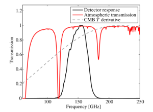
| B2_frequency_spectrum_20141216.txt | Text file containing the average bandpass of BICEP2, corresponding to Figure 11 of BICEP2 2014 II. |
History
3. BICEP2 2014 Release Figures from Papers
| BICEP2 2014 I: Detection of B-mode Polarization at Degree Angular Scales by BICEP2 | Download Bundle | ||
|---|---|---|---|
| T/Q/U maps |
|
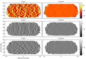
Figure 1: BICEP2 T, Q, U maps. The left column shows the basic signal maps with 0.25° pixelization as output by the reduction pipeline. The right column shows difference (jackknife) maps made with the first and second halves of the data set. No additional filtering other than that imposed by the instrument beam (FWHM 0.5°) has been done. Note that the structure seen in the Q and U signal maps is as expected for an E-mode dominated sky. | PDF / PNG |
| BICEP2 power spectrum results |
|
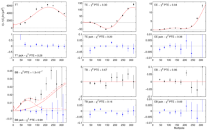
Figure 2: BICEP2 power spectrum results for signal (black points) and temporal-split jackknife (blue points). The red curves show the lensed-ΛCDM theory expectations while the dashed red curves show r = 0.2 tensor spectra and the sum of both. The error bars are the standard deviations of the lensed-ΛCDM+noise simulations and hence contain no sample variance on tensors. The probability to exceed (PTE) the observed value of a simple χ2 statistic is given (as evaluated against the simulations). Note the very different y-axis scales for the jackknife spectra (other than BB). See the text for additional discussion of the BB spectrum. (Note that the calibration procedure uses EB to set the overall polarization angle so TB and EB as plotted above cannot be used to measure astrophysical polarization rotation.) | PDF / PNG |
| E/B maps |
|
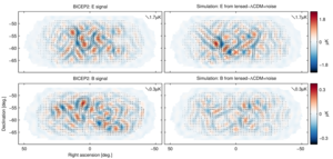
Figure 3: Left: BICEP2 apodized E-mode and B-mode maps filtered to 50 < ℓ < 120. Right: The equivalent maps for the first of the lensed-ΛCDM+noise simulations. The color scale displays the E-mode scalar and B-mode pseudoscalar patterns while the lines display the equivalent magnitude and orientation of linear polarization. Note that excess B mode is detected over lensing+noise with high signal-to-noise ratio in the map (s/n > 2 per map mode at ℓ ≈ 70). (Also note that the E-mode and B-mode maps use different color and length scales.) | PDF / PNG |
| Jackknife PTE distributions |
|
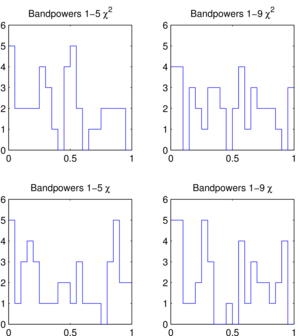
Figure 4: Distributions of the jackknife χ2 and χ PTE values over the 14 tests and three spectra given in Table 1. These distributions are consistent with uniform. | PDF / PNG |
| BB spectra from T-only simulations |
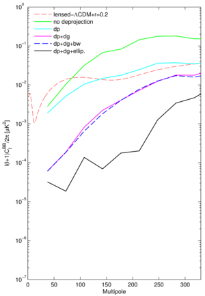
|
Figure 5a: BB spectra from T-only input simulations using the measured per channel beam shapes compared to the lensed-ΛCDM+r = 0.2 spectrum. From top to bottom the curves are (i) no deprojection, (ii) deprojection of differential pointing only (dp), (iii) deprojection of differential pointing and differential gain of the detector pairs (dp+dg), (iv) adding deprojection of differential beam width (dp+dg+bw), and (v) differential pointing, differential gain, and differential ellipticity (dp+dg+ellip). | PDF / PNG |
| Estimated levels of other systematics |
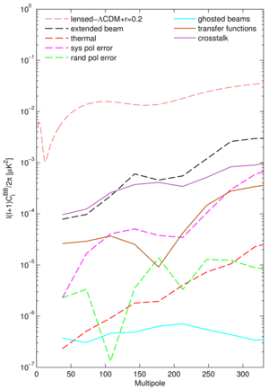
|
Figure 5b: Estimated levels of other systematics as compared to the lensed-ΛCDM+r = 0.2 spectrum. Solid lines indicate expected contamination. Dashed lines indicate upper limits. All systematics are comparable to or smaller than the extended beam mismatch upper limit. | PDF / PNG |
| Dust foreground projections |
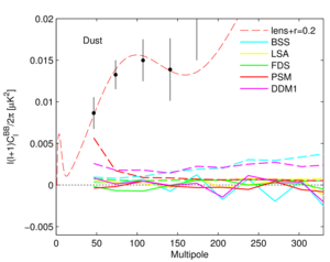
|
Figure 6a: Polarized dust foreground projections for our field using various models available in the literature, and a new one formulated using the information officially available from Planck. Dashed lines show autospectra of the models, while solid lines show cross spectra between the models and the BICEP2 maps. The BICEP2 auto spectrum from Figure 2 is also shown with the lensed-ΛCDM+r = 0.2 spectrum. | PDF / PNG |
| Synchrotron foreground constraints |
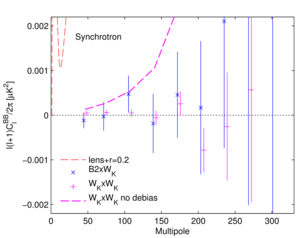
|
Figure 6b: Polarized synchrotron constraints for our field using the WMAP K band (23 GHz) maps projected to 150 GHz using the mean spectral index within our field (β = -3.3) from WMAP. The blue points with error bars show the cross spectrum between BICEP2 and WMAP maps, with the uncertainty estimated from cross spectra against simulations of the WMAP noise. The magenta points with error bars and the dashed curve show the WMAP auto spectrum with and without noise debias. | PDF / PNG |
| BICEP2 and BICEP1 cross-spectra |
|
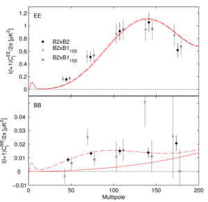
Figure 7: The BICEP2 EE and BB auto spectra (as shown in Figure 2) compared to cross spectra between BICEP2 and the 100 and 150 GHz maps from BICEP1. The error bars are the standard deviations of the lensed-ΛCDM+noise simulations and hence contain no sample variance on tensors. (For clarity the cross spectrum points are offset horizontally.) | PDF / PNG |
| Spectral index constraint |
|
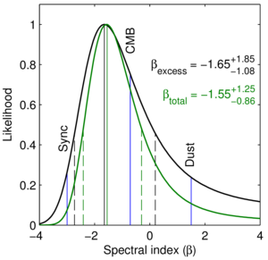
Figure 8: The constraint on the spectral index of the BB total signal (green) and excess signal over lensed ΛCDM (black), based on joint consideration of the BICEP2 auto, BICEP1100 auto, and BICEP2×BICEP1100 cross spectra. The curve shows the marginalized likelihood as a function of assumed spectral index. The vertical solid and dashed lines indicate the maximum likelihoods and the ±1σ intervals. The blue vertical lines indicate the equivalent spectral indices under these conventions for the CMB, synchrotron, and dust. The observed signal is consistent with a CMB spectrum, while synchrotron and dust are both disfavored. | PDF / PNG |
| Cross spectra of BICEP2 with BICEP1 and Keck Array |
|
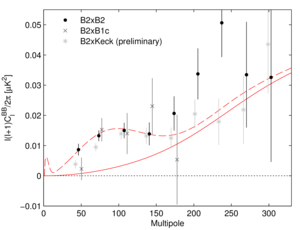
Figure 9: Comparison of the BICEP2 BB auto spectrum and cross spectra taken between BICEP2 and BICEP1 combined, and BICEP2 and Keck Array preliminary. The error bars are the standard deviations of the lensed-ΛCDM+noise simulations and hence contain no sample variance on tensors. (For clarity the cross spectrum points are offset horizontally and the BICEP2×BICEP1 points are omitted at ℓ > 200.) | PDF / PNG |
| Constraint on tensor-to-scalar ratio r |

|
Figure 10: Left: The BICEP2 band powers plotted with the maximum likelihood lensed-ΛCDM+r = 0.20 model. The uncertainties are taken from that model and hence include sample variance on the r contribution. Middle: The constraint on the tensor-to-scalar ratio r. The maximum likelihood and the ±1σ interval is r = 0.20+0.07-0.05, as indicated by the vertical lines. Right: Histograms of the maximum likelihood values of r derived from lensed-ΛCDM+noise simulations with r = 0 (blue) and adding r = 0.2 (red). The maximum likelihood value of r for the real data is shown by the vertical line. | PDF / PNG |
| Constraints on r when subtracting foreground models |
|
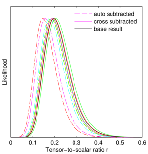
Figure 11: Modified constraints on the tensor-to-scalar ratio r when subtracting each of the foreground models shown in Figure 6 from the BICEP2 BB bandpowers. The line styles and colors match Figure 6 with dashed for auto spectra and solid for cross spectra. The probability that each of these models reflects reality is hard to assess—see the text for discussion. | PDF / PNG |
| Joint constraint on r and lensing scale factor |
|
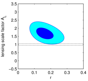
Figure 12: Joint constraints on the tensor-to-scalar ratio r and the lensing scale factor AL using BICEP2 BB band powers 1–9. One and two σ contours are shown. The horizontal dotted lines show the 1σ contraint from Planck Collaboration XVI (2013). The B-mode lensing signal is detected at 5.5σ, with an amplitude ∼2σ higher than the expected value. | PDF / PNG |
| Constraint on r and ns from BICEP2 and CMB temperature measurements if cosmological model is extended to allow running of the scalar spectral index |
|
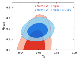
Figure 13: Indirect constraints on r from CMB temperature spectrum measurements relax in the context of various model extensions. Shown here is one example, following Planck Collaboration XVI (2013) Figure 23, where tensors and running of the scalar spectral index are added to the base ΛCDM model. The contours show the resulting 68% and 95% confidence regions for r and the scalar spectral index ns when also allowing running. The red contours are for the “Planck+WP+highL” data combination, which for this model extension gives a 95% bound r < 0.26. The blue contours add the BICEP2 constraint on r shown in the center panel of Figure 10. See the text for further details. | PDF / PNG |
| BICEP2 BB auto spectra and upper limits from previous experiments |
|
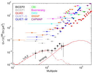
Figure 14: BICEP2 BB auto spectra and 95% upper limits from several previous experiments (Leitch et al. 2005; Montroy et al. 2006; Sievers et al. 2007; Bischoff et al. 2008; Brown et al. 2009; QUIET Collaboration et al. 2011, 2012; Bennett et al. 2013; Barkats et al. 2014). The curves show the theory expectations for r = 0.2 and lensed-ΛCDM. The BICEP2 uncertainties include sample variance on an r = 0.2 contribution. | PDF / PNG |
| BICEP2 2014 II: Experiment and Three-year Data Set | Download Bundle | ||
|---|---|---|---|
| BICEP2 mount and telescope diagram |
|
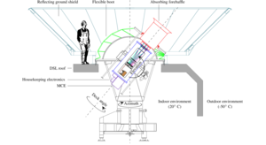
Figure 1: The BICEP2 telescope in the mount, looking out through the roof of the Dark Sector Laboratory (DSL) located 800 m from the geographic South Pole. The three-axis mount allows for motion in azimuth, elevation, and boresight rotation (also called “deck rotation”). An absorbing forebaffle and reflective ground screen prevent sidelobes from coupling to nearby objects on the ground. A flexible environmental seal or “boot” maintains a room temperature environment around the cryostat and mount. The telescope forms an insert within a liquid helium cryostat. The focal plane with polarization-sensitive TES bolometers is cooled to 270 mK by a 4He/3He/3He sorption refrigerator. The housekeeping electronics and Multi-Channel Electronics (MCE) attach to the lower bulkhead of the cryostat. | PDF / PNG |
| BICEP2 exterior photo |
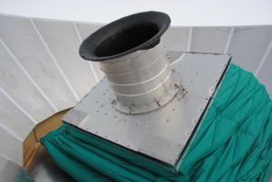
|
Figure 2: BICEP2 absorbing forebaffle, flexible environmental seal (the “boot”), and ground shield. The telescope and mount sit below the boot inside the Dark Sector Laboratory. | PDF / PNG |
| BICEP2 optical design |
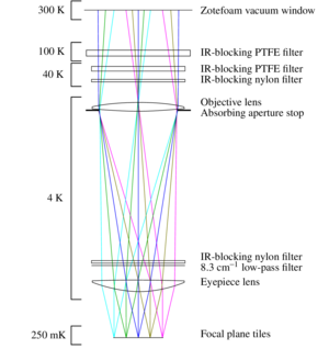
|
Figure 3: The telescope optical system. All components (except the window) have been anti-reflection coated to provide minimal reflection at 150 GHz. All optics below the 40 K nylon filter are cooled to 4 K, providing low and stable optical loading. Due in large part to the radially symmetric design, simulations predict well-matched beams for two idealized orthogonally polarized detectors at the focal plane. | PDF / PNG |
| Cross-section of the telescope insert |
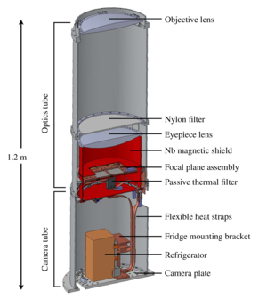
|
Figure 4: Cross-sectional view of the telescope insert. The entire telescope insert assembly is cooled to 4 K by a thermal link to a liquid helium bath. The optics tube provides rigid structural support for the optical chain, including the lenses, filters, and aperture stop. The camera tube assembly houses the sub-kelvin sorption refrigerator and the cryogenic readout electronics in a radiatively and thermally protected enclosure. The sub-kelvin focal plane assembly sits within a superconducting Nb magnetic shield. The focal plane is thermally connected to the fridge via a passive thermal filter. | PDF / PNG |
| Cross-section of sub-kelvin stages |
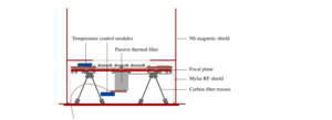
|
Figure 5: Cross-sectional view of the sub-kelvin hardware. The superconducting Nb magnetic shield is heat-sunk to 350 mK. Within, the focal plane is isolated from thermal fluctuations by eight carbon fiber legs. A thin aluminized Mylar shroud extends from the top of the focal plane assembly to the bottom of the Nb magnetic shield to minimize radio frequency pickup. Temperature stability is maintained through the combined use of active and passive filtering. The passive thermal filter, on the bottom of the focal plane, serves to roll off thermal fluctuations at frequencies relevant to science observations, while active temperature control modules maintain sub-millikelvin stability over typical observation cycles. | PDF / PNG |
| Focal plane assembly |

|
Figure 6: The assembled focal plane on the carbon fiber truss structure and 350 mK Nb plate. The four anti-reflection tiles and detector tiles sit beneath square windows in the copper plate. This assembly will be covered in the aluminized Mylar radio frequency shield, with a square opening only above the detector tiles. Left: Unshielded assembly; Left inset: Corrugations in the edges of the copper plate next to the detector tiles; Right: The underside of the focal plane Cu plate, with detector tiles and SQUID and Nyquist chips mounted. | PDF / PNG |
| Focal plane exploded view |
|
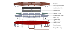
Figure 7: Exploded view of the layers of the focal plane. The Cu plate forms the substrate on which everything else is assembled. The detector tiles are pressed against antireflection tiles and look out through four square cutouts in the Cu plate with corrugated edges. The TES detectors and antennas are on the bottom surface of the tile, so that radiation passes through the Si wafer before reaching the slot antennas. A layer of Metglas magnetic shielding sits between the Cu plate and the printed circuit board (PCB). The PCB layer routes electrical traces between the detector tiles, multiplexing (MUX) chips, and micro-D connectors, and acts as a base for wire-bonding the tiles. The MUX chips sit on alumina carriers that mate to the PCB. The Nb backshort is held at a distance of one quarter wavelength from the tiles by Macor spacers. It is attached last to sandwich the circuit board, MUX chips, and tiles. | PDF / PNG |
| Close-up of BICEP2 pixel |
|
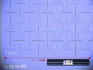
Figure 8: Partial view of one BICEP2 dual-polarization pixel, showing the band-defining filter (lower left), TES island (lower right), and part of the antenna network and summing tree. The vertically oriented slots are sensitive to horizontal polarization and form the antenna network for the A detector, while the horizontally oriented slots receive vertical polarization and are fed into the B detector. In this way the A and B detectors have orthogonal polarizations but are spatially co-located and form beams that are coincident on the sky. This view corresponds to a boresight angle of 90°. At boresight angle of 0° the A detectors receive vertical polarization and the B detectors receive horizontal polarization. | PDF / PNG |
| Band-defining filter |
|
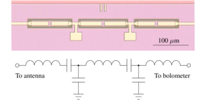
Figure 9: 150 GHz band-defining filter and equivalent circuit. Each filter consisted of three inductors in series, coupled to each other through a T-network of capacitors. | PDF / PNG |
| TES island |
|
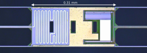
Figure 10: TES island for a single BICEP2 detector. The island was supported by six lithographically etched legs. Microwave power, entering from the left, terminated into a resistive meander. The deposited heat is measured as a decrease in electrical power (or current) dissipated in the titanium TES, which appears as a blue rectangle on the right of the island. The TES voltage bias was provided by two micro-strip lines at right. To increase the dynamic range of the device, an aluminum TES (seen as a white rectangle below the titanium film) was deposited in series with the titanium TES, providing linear response across a wide range of background loading conditions. The heat capacity of the island was tuned by adding 2.5 μm thick evaporated gold, which is distributed across the remaining real estate of the island. This made the detector time constants slow enough for stable operation. | PDF / PNG |
| BICEP2 frequency response |
|
Figure 11: The array-averaged frequency response spectrum (black solid line). Atmospheric transmission from the South Pole (red solid line) and the CMB anisotropy (gray dashed line) are also shown for comparison. The BICEP2 band center is 149.8 GHz and the bandwidth is 42.2 GHz (28%). The detector response and CMB spectra are normalized to unit peak, and the atmospheric transmission spectrum is in units of fractional power transmitted. | PDF / PNG |
| Histograms of bolometer properties |
|
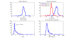
Figure 12: Histograms of measured bolometer properties per detector. Top left: Optical efficiency. This measurement was taken in lab with a beam-filling source. It was converted to an efficiency number using the measured spectral bandwidth of 42 GHz. Top right: Thermal conductance of the legs. Two of the tiles have Gc ≈ 100 pW/K and two have higher Gc ≈ 140 pW/K. Bottom left: Time constants with 2011–12 biases. The vertical dashed line shows the median of the distribution, 0.9 ms. These time constants are taken from raw-mode data in which the MCE and GCP digital filters have not been applied. Bottom right: Noise equivalent temperature per detector with 2011–12 operating parameters. NET is shown for the 2011–12 operating parameters. | PDF / PNG |
| TES resistance vs temperature |
|
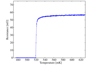
Figure 13: Example resistance vs. temperature characteristic for a JPL TES detector. The resistance rises from zero to 90% of the normal state resistance within 5 mK. | PDF / PNG |
| Per-tile noise equivalent temperature |
|
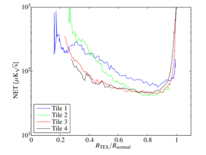
Figure 14: Per-tile noise equivalent temperature (NET) in units of CMB temperature as a function of the detector resistance. These data were taken under conditions of low atmospheric loading during the winter of 2010 and used to select new TES bias values to improve the instrumental sensitivity. NET sharply increases at the top of the superconducting-normal transition (high RTES/Rnormal) as the detectors saturate. In BICEP2 the NET also increases in the middle and lower part of the transition because of TES excess noise. The excess noise increases with increasing transition steepness β, which is larger at low fractional resistance. Note that the minima of the NET curves shown here do not directly represent the final noise level of BICEP2 after optimization, for several reasons. The NET values have been approximately converted to CMB temperature units assuming a typical value of the sky temperature at zenith. Variation in sky temperature will therefore affect the minimum NET as plotted, but does not impact the selection of optimal bias point. The NET as optimized is somewhat better than shown because the TES bias is configured per column rather than using a single value for each tile. Finally, the 2010 data shown here do not use the improved 2011–12 multiplexing configuration. | PDF / PNG |
| Time constants and transfer functions |
|
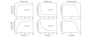
Figure 15: Measured time constants and transfer functions for a typical detector (top) with time constant τ < 1 ms and a slow detector (bottom) with time constant τ ≈3 ms. The three panels show a rising edge, falling edge, and a transfer function measured with a square-wave-modulated microwave source as described in the text. Step responses are normalized to the step size, and transfer functions are normalized to unit gain at the 10 Hz modulation frequency of the data. The blue curves are data. For the time constant panels, the red dashed lines are a fit to a single-exponential rise and fall with time constants as indicated. For the transfer function panels, the red dashed curve is the transfer function of the MCE and GCP digital filters alone. For fast detectors such as the one in the top panel, the data match this profile to within 0.5%, with no evidence of additional time constants. The MCE and GCP digital filters have not been applied to the raw-mode time constant data shown in the left and center panels. All data shown use the 2011–12 bias and multiplexing settings. | PDF / PNG |
| Measured noise spectrum |
|
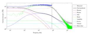
Figure 16: Measured noise spectrum of a characteristic detector under typical observing conditions and with 2010 readout settings. Also shown are modeled noise components estimated from measured detector parameters. The measured noise is well described by the sum of individual noise model components at low frequencies, where the scan-modulated science signal peaks. Due to the limited bandwidth of the detector readout (indicated by the dashed vertical line), aliased excess noise contributes non-negligibly to the achieved noise performance at low frequencies. For the 2011 and 2012 observing seasons, the increase in multiplexing rate from 15 kHz to 25 kHz reduced the aliased noise to approximately half its original level. | PDF / PNG |
| Stacked far-field beam map |

|
Figure 17: A map of the BICEP2 far-field response made with the thermal source in units of log10(power), showing dynamic range of more than six decades. Beam maps for individual detectors are shifted to align the peaks and coadded over all operational detectors. The measured shape of the main beam and Airy ring structure are well matched by simulations, as shown in the Beams Paper. Crosstalk features are apparent as small additional beams to the left and right, at a low level relative to the main beam strength. The dark feature near the bottom is negative-going crosstalk found only in a subset of channels. | PDF / PNG |
| Far-field beam characterization |

|
Figure 18: Results of far-field beam characterization with a chopped thermal source. Left: Typical measured far-field beam on a linear scale. Middle: The Gaussian fit to the measured beam pattern. Right: The fractional residual after subtracting the Gaussian fit. Note finer color scale in the right-hand differenced map. | PDF / PNG |
| Polarized response of a detector pair |
|
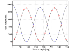
Figure 19: Polarization response of a detector pair from a rotating polarized source measurement. The x-axis shows the source polarization angle relative to the vertical. The A detector (blue points) responds to vertical polarization and the B detector (red points) responds to horizontal polarization at a boresight angle of 0°. The cross-polar signal is ∼0.5%, consistent with the level of crosstalk. The small deviation from a sinusoidal form is caused by variation in source illumination of the telescope, included in the fit curves. | PDF / PNG |
| BICEP2 observing fields |
|
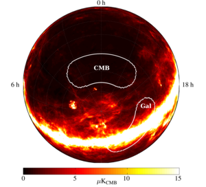
Figure 20: BICEP2 observing fields relative to the polarization amplitude predicted from FDS (Finkbeiner et al. 1999) model 8, assuming a 5% polarization fraction. | PDF / PNG |
| BICEP2 observing pattern |

|
Figure 21: Observing pattern of a typical three-day schedule. The scansets of Phase G are numbered, with the first scanset at the lowest elevation. The first scanset of Phase G is shown in bold, showing the throw of the field scans (horizontal line) and the bracketing elevation nods (vertical line). The two six-hour phases can vary in elevation: the Galactic D phase is shown at the lowest of four elevation steps, and the CMB G phase is shown at the lowest of three elevation steps. The H and I phases on the third LST day alternate between the B/C pattern and the E/F pattern. | PDF / PNG |
| Average noise power spectra |
|
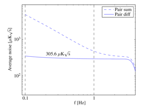
Figure 22: Average noise power spectra of all detector pairs with 2011–12 settings. Cuts and inverse-variance weighting are applied as in standard mapmaking. The pair-sum spectra show 1/f noise, which is removed by taking the pair difference. The average NET per detector is taken from the average power spectral density in the pair-difference spectrum between 0.1 and 1 Hz. | PDF / PNG |
| Three-year live time, sensitivity, and map depth |
|
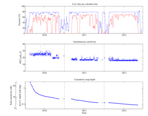
Figure 23: Integration of the BICEP2 three-year data set. Top panel: Time per day spent in CMB scans, regular calibrations, and refrigerator cycling. During austral summers (November–February), observing schedules have been interspersed with beam mapping and other tests and calibrations. During the austral winter, on-source efficiency (including Galactic observations) has been high, never falling far below the ideal 79.2% in the 2012 observing season. The lower, red curve includes data quality cuts. Middle panel: Mapping speed over time. The improvement from early to late 2010 is caused by the optimization of TES biases, the improvement from 2010 to 2011 is caused by the change to 25 kHz multiplexing, and the small improvement from 2011 to 2012 was caused by a small increase in the number of active channels. Each data point represents one observing phase of six or nine hours, as described in Section 12.3. Bottom panel: Cumulative map depth over time as calculated in §14.2. | PDF / PNG |
| Polarization and coverage maps |
|
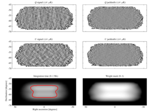
Figure 24: Polarization maps and coverage maps used to calculate map depth (color scales in parentheses). The maps are Stokes Q and U in the three-year data set, with full coadds on the left and differenced chronological jackknife maps on the right. The Q maps show a horizontal and vertical pattern, while the U maps show a diagonal pattern, together revealing the dominant E-mode polarization of the CMB. The jackknife maps contain no signal but only noise. They are used to calculate the depth in our polarization maps. The lower left panel shows the integration time per 0.25°×0.25° pixel and the 70% contour used in the older definition of the map depth, while the lower right panel shows the variance-weight map used in the definition adopted here. | PDF / PNG |